High-Order Statistics of Temperature Fluctuations in an Unstable Atmospheric Surface Layer over Grassland

Rui LYU,Fei HU,Lei LIU,Jingjing XU,and Xueling CHENG

1State Key Laboratory of Atmospheric Boundary Layer Physics and Atmospheric Chemistry,Institute of Atmospheric Physics,Chinese Academy of Sciences,Beijing 100029,China

2University of Chinese Academy of Sciences,Beijing 100049,China

ABSTRACT Skewness(S)and kurtosis(K)of temperature in the surface layer over a grassland are investigated under unstable thermal stratifications.We find that both skewness and kurtosis generally obey Monin–Obukhov similarity theory and tend to be constant values(1.5 and 5.3,respectively)when the stability parameter z/L<−2.Quantitative formulas of the similarity functions are proposed.The temperature probability density function(PDF)is close to Gaussian in near neutral stratification and non-Gaussian in unstable stratification.The in fluence of coherent motions on the PDF behavior is analyzed using the quadrant analysis technique.It shows that PDF behaviors are controlled by ejections and sweeps.The results also indicate that the PDF type of the ejections always follows a Gaussian distribution,while the PDF of the sweeps changes with stability.

Key words:temperature fluctuations,Monin–Obukhov similarity theory,skewness,kurtosis

1.Introduction

Research on probability density functions(PDFs)of scalars in the atmospheric boundary layer is mainly driven by boundary layer modeling and turbulence diffusion simulation.Theoretically,any order closure of the Reynolds equation can be performed with specific PDFs.Several forms of scalar PDF have been proposed,including beta distribution(Graf et al.,2010),pareto distribution(Schop flocher and Sullivan,2002)and so on(Price,2001).So far,no consensus has been reached on the scalar PDF due to its non-Gaussian property and complexity.Therefore,high-order moments of scalars attract more attention instead,because they can reflect the characteristics of probability density to a certain extent.Skewness and kurtosis,which are the third and fourth standardized moments,are most commonly used both in theoretical analysis(Schop flocher and Sullivan,2005;Nironi et al.,2015)and modeling(Gryanik and Hartmann,2002;Bisignano et al.,2017).Skewness is considered to have relevance to non-local transport,while kurtosis reveals microstructures and processes in turbulence(Quan et al.,2012).

The scalar temperature has been widely investigated because of its importance in the surface layer.Research on temperature fluctuations have mainly focused on secondorder moments,such as sensible heat flux(Quan and Hu,2009;Zuo et al.,2009;Wang et al.,2013).So far,few works have reported on high-order moments of temperature fluctuations(Tillman,1972;Antonia et al.,1981;Afanas’ev et al.,1999).Arguments on whether the behavior of temperature skewness can be predicted by Monin–Obukhov similarity theory(MOST)over horizontal homogeneity existed in the early days(Monin and Yaglom,1971;Businger,1973).Later,observation confirmed that MOST is applicable to temperature skewness(Tillman,1972;Antonia et al.,1981;Andreas et al.,1998).Unfortunately,the relationship between skewness and stability obtained from these observations was based on a small amount of data,indicating the applicability of the above theory to be limited.Moreover,to the best of our knowledge,a quantitative relationship between kurtosis and stability has not yet been established,and to establish such a relationship is one of the main purposes of this paper.On the other hand, it has been widely recognized that the joint probability distribution of vertical velocity and temperature is closely related to coherent motion(Katul et al.,1997).Ejection and sweep motions are considered to be the two major types of coherent eddies.A third-order cumulative expansion of the joint probability distribution,which contains the information of skewness,is often used to predict the difference between flux contributions due to ejection and sweep mo-tions(Nakagawa and Nezu,1977;Katul et al.,1997).Moreover,how atmospheric stability affects coherent motion still attracts much attention(Wang et al.,2013),and an in-depth understanding of coherent motion will help to establish a refined PDF.All these issues are discussed.

In this work,we investigate temperature fluctuations in the surface layer over grassland under the framework of similarity theory.There are two main purposes to the paper.One is to set up a quantitative relationship between the stability parameter and high-order statistics of temperature.The other is to investigate the influence of coherent motions on temperature’s PDF.The paper is organized as follows:In section 2,the experimental design and data processing are described.In section 3.1,we discuss the applicability of MOST to third and fourth-moments of temperature.Then,we derive the similarity functions of skewness and kurtosis in section 3.2.In section 3.3,the behavior of the fine structure of the PDF and its relationship with coherent motions is presented using the quadrant analysis technique.Finally,a conclusion is provided in section 4.

2.Data and processing

2.1.Experiments and instruments

The data are derived from the grass-covered boundary layer experiment carried out in the northeast of Xilin Hot(44.124°N,116.29°E),Inner Mongolia,China.A 100-m tower stands over sufficiently flat and uniform grassland,at an altitude of 1159 m(Fig.1a).The entire experiment began in May 2009 and ended in April 2010.Both slow-and fastresponse instruments are installed on the tower(Fig.1c).The instruments and their placement heights are shown in Table 1.

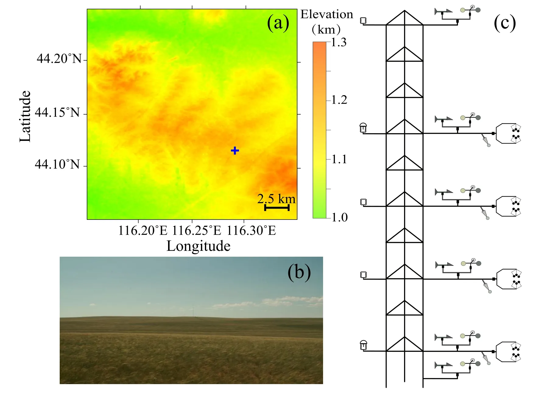
Fig.1.Basic information about the experiment:(a)topographic map(using ASTER Global Digital Elevation Model data)surrounding the observation site(indicated by the plus symbol);(b)photograph near the observation site during July 2009;(c)sketch of the 100-m tower and instruments.

Three months(June to August 2009)of data were analyzed.During this period,large areas of ground were covered by dozens of centimeters of grass(Fig.1b).The data used for turbulence calculation are derived from 10,30 and 50 m.Although the height of 50 m is in the upper atmospheric surface layer,sometimes exceeding the surface layer,we still use data at this height for obtaining more near-ground information(Garai et al.,2013).Weak(<3 m s−1)and moderate(3–12 m s−1)intensity winds exist in all directions,with only small amounts of strong winds(＞ 12 m s−1)(Fig.2).

2.2.Data processing

We begin by de fining some symbols used in this study.u,v and w are the longitudinal,lateral and vertical velocity components,while T is the air temperature.The turbulent fluctuations are computed following X′=X−,where X is any variable,the overbar denotes the time averaging operator and the primed variable denotes the turbulent part.

Before analysis,sonic temperature correction is performed to exclude the impact of water vapor using the rela-tionship Ts=T(1+0.51q),where Tsis the sonic temperature and q is the specific humidity(Schotanus et al.,1983).

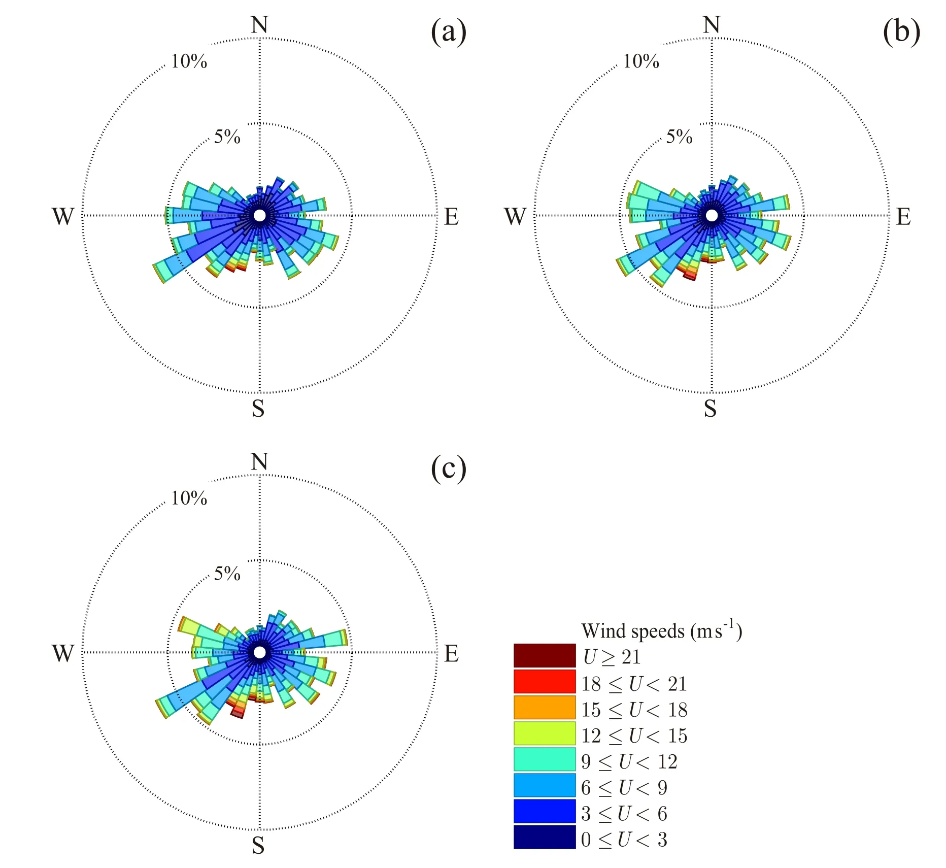
Fig.2.Wind roses at three levels for the analyzed period using vanes data:(a)10 m;(b)30 m;(c)50 m.U represents the speed observed by vanes.

2.2.1. Averaging time

The choice of averaging time is a significant consideration when calculating the turbulence statistics.When a short averaging time is chosen,the statistics may exclude the contributions by turbulent motions in some scales.When an averaging time that is too long is chosen,the statistics may include the contributions by non-turbulent motions,such as mesoscale motions(Mahrt,2010).

There are several methods that are often used in the selection of the averaging time.Lenschow et al.(1994)discussed the selection of averaging time from the perspective of error analysis.They pointed out that the statistical error of estimating the moment decreases as the averaging time increases for the stationary stochastic process.When the averaging time is much larger than the integral time scale,the error is mainly determined by the random error,which represents the random scatter of sampling.Specially,for a Gaussian process,once the averaging time tais chosen,the random error of the time mean of the nth-order central moment can be expressed by an(τ/ta)1/2,where τ is the integral time scale and anis a coefficient that increases with the increasing of order n.It indicates that a longer averaging time is needed to reduce the random error.However,the calculation of the integral time scale τ still depends on the averaging time(Yu et al.,2008;Varshney and Poddar,2011),which makes this rule not so effective to determine the averaging time.

Another method of determining the averaging time,often used in micrometeorology,is the ogive test(Desjardins et al.,1989).This method is based on analysis of the secondorder mixed moment of vertical velocity and temperature.It calculates the cumulative integral of the cross-spectral turbulent flux,expressed asCow′T′(f)df,where Co is the cross spectrum and f0is the cut frequency.The averaging time is acceptable when the integration is close to a constant at low frequencies.An interval of 30 minutes is usually determined using this method(Foken et al.,2006).This interval has also been used in some studies on high-order moments of turbulent fluctuations(Jacobs et al.,2001).In this study,we employ an averaging time of 30 minutes.Averaging times of 15 minutes and 1 hour were also used for comparison and no significant differences existed,as shown in section 3.1.

2.2.2.Quality control and coordinate rotation

Data quality control is performed as follows:

(1)Periods of relative humidity greater than 70%are removed to avoid the impact of potential precipitation.

(2)Spikes,amplitude resolution problems,dropouts and discontinuities are detected following Vickers and Mahrt(1997).A threshold of 5 times the standard deviation is chosen when detecting spikes in this study,instead of 3.5 times the standard deviation in the original literature to preserve more information in PDF tails for non-Gaussian distributions.

(3)Thresholds are given as Vickers and Mahrt(1997)and Klipp and Mahrt(2004)recommended.The absolute limit for horizontal wind is 30 m s−1and for temperature it is −30°C to 50°C.The critical value for vertical gradients of mean velocity is 0.001 s−1.

Detrending and coordinate rotation are carried out after the above steps.We simply use the linear detrending approach(Kaimal and Finnigan,1994).Coordinate rotation has no impact on calculation of high-order moments of temperature.But,it will influence calculation of the sensible heat flux and stability parameter.The most commonly used methods are the double rotation and planar fit methods(Wilczak et al.,2001).Before analysis,both methods were tested to calculate fluxes and no significant differences were found.The correlation coefficient of heat fluxes using these two methods exceeds 0.99 at each height.We only show the results with double rotation in the following part of the paper.Since linear detrending and double rotation are linear transformation methods,exchanging their operation orders does not affect the results.

2.2.3.Stationarity

Stationarity is a fundamental assumption in the statistical computation of turbulence and similarity theory analysis(Wyngaard,2010).When the turbulence is stationary,the time-average statistics will be equal to the ensembleaverage statistics,which is also called ergodicity.Strictly speaking,turbulence in the atmospheric boundary layer has always been in a non-stationary state,which makes it hard to select an appropriate criterion of stationarity.Vecenaj and De Wekker(2015)compared several approaches of detecting non-stationarity and concluded that no single approach is most suitable for detecting non-stationarity of first-and second-order moments of atmospheric time series.They did,however,point out that the criterion proposed by Foken and Wichura(1996)performed better than other criteria in their investigation.This criterion detects the non-stationarity of second-order moments w′T′).Together with detrending,it can screen out the stationary time series effectively.Most intervals(more than 80%in our research)passing the test are still stationary when applying this approach to skewness and kurtosis.

After the above treatments,about 15%to 25%of the periods remain at each level(Table 2).We did not carry out an uncertainty assessment because it would have reduced the intervals that could be analyzed(Stiperski and Rotach,2016).All the following analysis is based on intervals under unstableconditions.

3.Methods and results

3.1.Similarity relationship of third-and fourth-order moments

As skewness and kurtosis are the normalized third-and fourth-order moments,we first investigate the behaviors of third-and fourth-order moments under unstable conditions.

According to MOST,the scaled mean variable at the height of z in the surface layer is the only function of the dimensionless stability parameter ζ:

Table 2.Number of 30-minute intervals after quality control and stationarity testing within the three-month period at each level.[Total:the number of all intervals.After quality control:the number of intervals after quality control.Stable/Unstable:the number of stable/unstable intervals(quality controlled)after stationary testing.]

where L is the Obukhov length,de fined by

In Eq.(2),θvis virtual potential temperature;is the friction velocity;is the kinematic heat flux;κ is the von Karman constant(0.4 in this article);and g is the gravitational acceleration(9.8 m s−2in this article).The subscript s represents the ground value.In this article,we regard the value at 10 m as the near ground value.Virtual potential temperature used in this work can be computed as θv≈Tv+gz/Cp=Ts+gz/Cp,where Tvis virtual temperature and close to Ts(Stull,1988)andCpis the specific heat for air at constant pressure(1005 J kg−1K−1in this paper).

According to Kader and Yaglom(1990),high-order moments of temperature fluctuations in an unstably stratified boundary layer,where thermal production should be taken into account,follow

In Eq.(3),ϕnrepresents a set of universal similarity functions.the temperature scale in surface layer.The value of n should be greater than or equal to 2.Cnis the coefficient determined by experiment.

Another form often used can be written as(De Franceschi et al.,2009)

where αnand βnare the corresponding coefficients.

When ζ→ −∞,Eq.(4)is consistent with Eq.(3)and we haveWhen ζ→ 0,which means the thermal stratification is near neutral in condition,Eq.(4)tends to be a constant with a value of αn,while Eq.(3)tends toward infinity.We use the form of Eq.(4)to fit the similarity function of temperature fluctuations.

Figure 3 shows non-dimensional high-order moments versus the Monin–Obukhov stability parameter ζ.The fitting results using Eq.(4)are also shown in the figure.Under unstable conditions,high-order(at least fourth-order)moments of temperature obey MOST.Non-dimensional similarity functions of second-,third-and fourth-order moments are given as:

Most existing studies focus only on the relationship between the second-order moment (often in the form of standard deviation)of the temperature and the stability parameter. Whenother earlier studies(Wyngaard et al.,1971).Very few studies about third-and forth-order moments can be found within the framework of similarity theory.When ζ→ −∞,we havewhich is smaller than the value given by Kader and Yaglom(C3=2 in their work).So far,according to our research,there is no literature on the accurate relationship between fourth-order moments and the stability parameter.The relationship between the fourth-order moments and the stability parameter shows

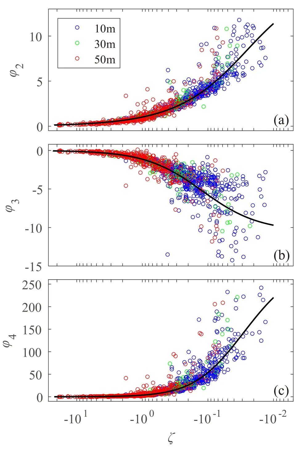
Fig.3.Non-dimensional high-order moments of temperature as functions of the Monin–Obukhov stability parameter for 10 m(blue circles),30 m(green circles)and 50 m(red circles):(a)second-order moment;(b)third-order moment;(c)fourth-order moment.Solid lines correspond to Eq.(5).

3.2.Similarity relationship of skewness and kurtosis

Under unstable conditions,we can express skewness(S)and kurtosis(K)as

Mathematical symbol〈〉means ensemble average.There is a negative sign in Eq.(6)because T∗is negative in unstable conditions.Equations(6)and(7)indicate that the behaviors of S and K are controlled by non-dimensional second-,third and forth-order moments.If second-,third-and fourth-order moments obey MOST,it can be expected that S and K obey MOST.

Figure 4 shows S and K as functions of the stability parameter.Though data points are scattered compared to those in Fig.3,S and K generally obey MOST.When ζ→ 0,S approaches zero and K approaches three.This implies that the PDF of temperature tends to be Gaussian when thermal stratification is close to neutral.As ζ decreases,S and K increase.Both S and K seem to get near-constant values in strongly unstable condition(ζ< −2).That S approaches a constant in very unstable conditions has also been found by other studies.However,different constants are given by different researchers:0.82 for Andreas et al.(1998);1 for Wyngaard and Sundararajan(1979);and 1.3 for Li and Bou-Zeid(2011,their Fig.11).All these values seem to be smaller compared with our result,which approximately equals to 1.5.The constant for K in very unstable conditions(ζ< −2)approximately equals 5.3 in our investigation.Results using an averaging time of 10 minutes and 1 hour are also shown in Figs.4c–f.No significant difference is found when using different averaging times.

One notable phenomenon is that lines deduced from Eq.(5)fail to predict an accurate relationship between S(or K)and ζ.The main reason is that the form of Eq.(4)is only an approximation.The coefficient and the form of Eq.(4)may change in different thermal stratification when buoyancy forces and dynamic forces change(Kader and Yaglom,1990).The error is further amplified when Eq.(4)is used to derive skewness and kurtosis.In order to give a more precise function,we directly fit the S and K.Notice that the solid line in Fig.4a describes the trend of the scattered points well.Thus,we slightly modify the form derived from Eqs.(5a)and(5b)and give the following form:

where a and b are coefficients determined by observation.

The solid line in Fig.4b deviates from observed K considerably and a new form is needed to fit the data.A square relationship has always been found between S and K in scalars(Graf et al.,2010;Quan et al.,2012).A similar behavior is also found in our investigation.This inspired us to suggest that the following function may be a good approximationwhen describing the relationship between kurtosis and the stability parameter:

Fig.4.Skewness(S)and kurtosis(K)as functions of the Monin–Obukhov stability parameter ζ for 10 m(blue circles),30 m(green circles)and 50 m(red circles),using different averaging times:(a,b)30 min;(c,d)10 min;(e,f)1 h.Solid lines are deduced from Eq.(6)and Eq.(7).

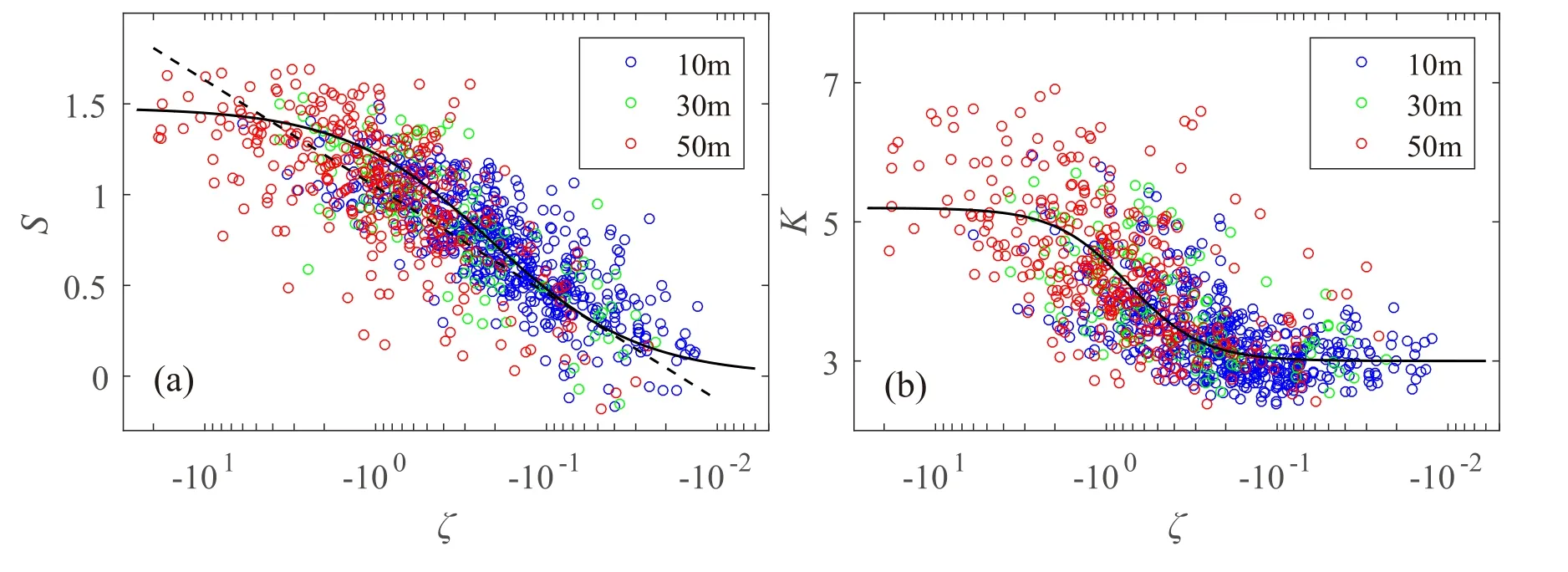
Fig.5.Fitted results of(a)skewness and(b)kurtosis.Solid lines correspond to Eq.(10).The dotted line,from Andreas et al.(1998),follows S=0.255ln(−ζ)+1.044.

where c,d and e are coefficients.We set c=3,as we find the kurtosis approaches 3 in neutral stability conditions.

Fitting Eqs.(8)and(9)to data,we have

The fitted curves are shown in Fig.5,together with the fitted result used by Andreas et al.(1998).The two forms of curves agree with each other on the trend,as shown in Fig.5a.However,the linear form used by Andreas et al.(1998)failed to predict the constants of skewness in near neutral and very unstable conditions.

Since skewness and kurtosis can be predicted by similarity theory,we speculate that the PDF of temperature also follows MOST.Figure 6 validates this idea.The PDF of normalized temperature fluctuations changes systematically with the stability parameter.In unstable conditions,the temperature PDF shows a non-Gaussian property.As the instability increases,the left tail of the temperature PDF becomes shorter and the right tail becomes longer,which has also been found by Liu et al.(2011).The skewness(0.04,0.32,0.86,1.22,1.43 for each PDF)and kurtosis(3.01,3.04,3.45,4.72,5.11 for each PDF)increase with the increase in instability.Moreover,the peak value of the PDF increases as the instability increases.The shape of the PDF is consistent with experimental results carried out near a wall in the laboratory(Emran and Schumacher,2008).We discuss the fine structures of these non-Gaussian PDFs in the next part.

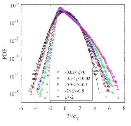
Fig.6.Normalized PDFs of temperature under different unstable conditions.The solid line is the Gaussian distribution curve.Data from 10 m,30 m and 50 m are all used here.

3.3.Relationship between coherent motions and PDFs of turbulent temperature fluctuations

In this section we study the relationship between coherent motions and the fine structure of the temperature PDF.Quadrant analysis,which has been widely used in studying coherent motions(Katul et al.,2006;Katsouvas et al.,2007;Wang et al.,2013),is performed in this section.Under unstable thermal stratification,according to the sign of the fluctuations of temperature and vertical velocity,the movements can be divided into four quadrants:

Quadrant 1:w′＞ 0,T′＞ 0,ejection

Quadrant 2:w′<0,T′＞ 0,inward interaction

Quadrant 3:w′<0,T′<0,sweep

Quadrant 4:w′＞ 0,T′<0,outward interaction

Based on this definition,the PDF of normalized temperature fluctuations can be decomposed into four parts:

where,f(T′)is the PDF of normalized temperature fluctuations and f(w′,T′)is the joint PDF of normalized vertical velocity and temperature;the subscript represents the respective quadrant.

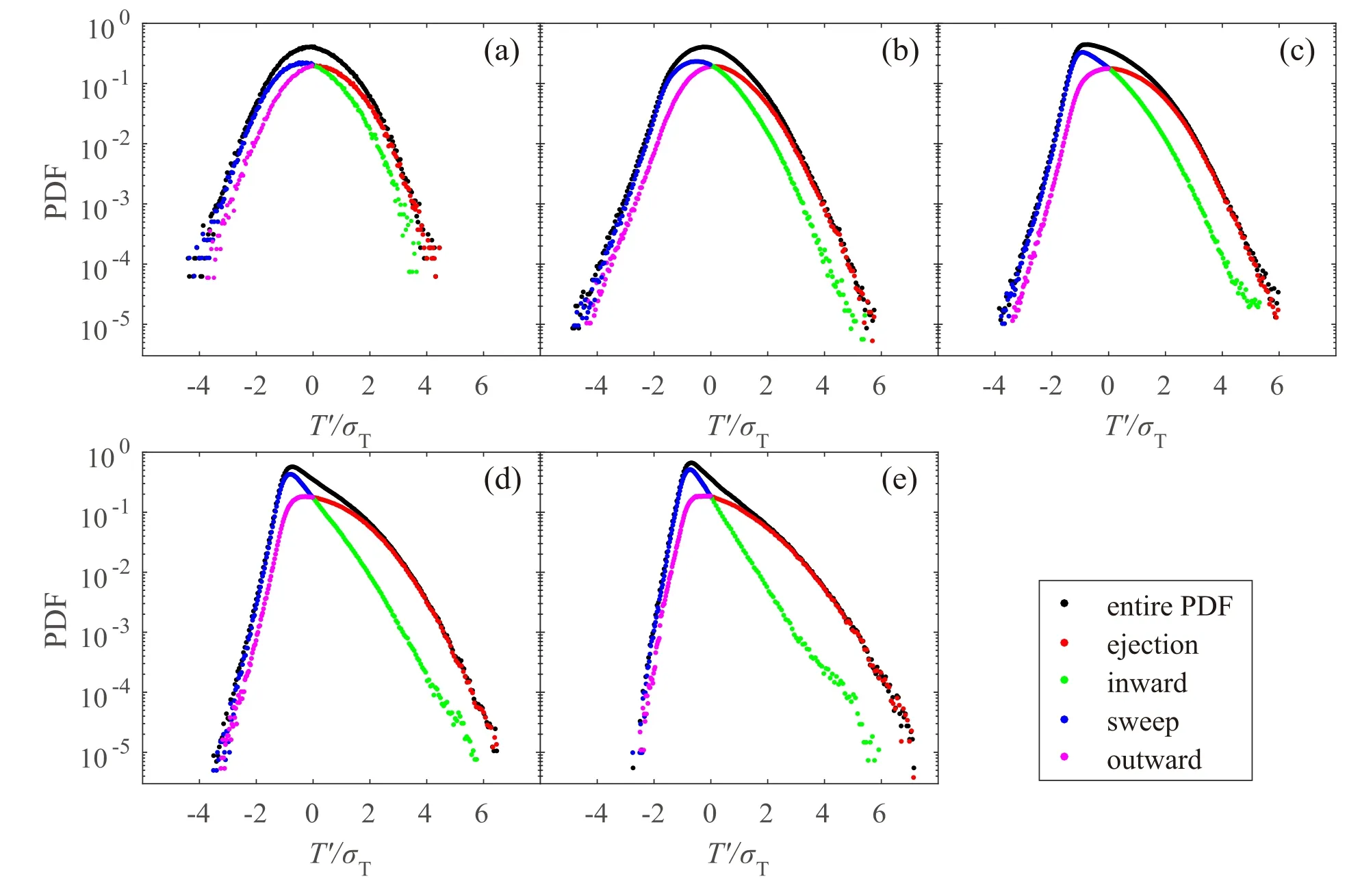
Fig.7.Quadrant compositions of PDFs under different unstable conditions:(a)−0.02< ζ<0;(b)−0.1< ζ< −0.02;(c)−0.5<ζ<−0.1;(d)−2<ζ<−0.5;(e)ζ<−2.Black dots represent entire PDFs.Dots with different colors represent contributors of each quadrant to PDFs.

Equation(11)decomposes the temperature PDF into contributions of ejections,inward interactions,sweeps and outwardinteractions.Figure 7 shows the result of PDF decomposition.For all conditions with different stabilities, the left tails of entire temperature PDFs coincide with those of sweeps’PDFs,while the right tails of entire temperature PDFs coincide with those of the ejections’PDFs.This indicates the left tail of the temperature PDF is mainly controlled by the sweep motions and the right tail of the temperature PDF is mainly controlled by ejection motions.Meanwhile,the peaks of sweeps’PDFs correspond to the peaks of entire temperature PDFs for ζ< −0.5.To illustrate how the temperature PDF changes systematically with stability,we analyze the influence of the stability parameter on the behaviors of ejections and sweeps.The contribution rate of each quadrant to temperature variance can be de fined as:

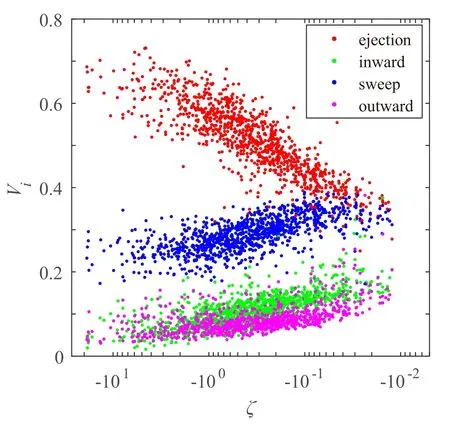
Fig.8.Contribution rate of each quadrant to temperature variance Vias a function of the stability parameter,where the contribution rate Viis calculated by summing up the squares of the normalized T′in the respective quadrants.

where Videnotes the contribution rate of the ith quadrant to variance(i=1,2,3,4).Since the variance of normalized temperature fluctuations is 1,the sum of Viequals 1.Figure 8 shows the contribution rate of each quadrant.Under unstable thermal stratification,ejections and sweeps contribute most of the temperature variance(more than 70%).When the thermal stratification is near neutral(−0.02<ζ<0),the contributions of ejections and sweeps are almost equal.With the increase in instability,the contribution of ejections increases while the contribution of sweeps decreases.Since large variance relates to large deviation(or amplitude),the amplitude of the ejections increases with the increase in instability,and the amplitude of sweeps decreases with the increase in instability.This explains why the left tail of the PDF becomes shorter and the right tail becomes longer when the stratification becomes more unstable(as shown in Fig.6).The PDFs of ejections and sweeps become more asymmetrical with the increase in instability.As a result,the skewness becomes larger.

We further study the time fraction of each quadrant,which is given by

where Diis the time fraction of the ith quadrant and Iiis an indicator function,expressed by

We focus on D1and D3,which are measures of time fractions of ejection and sweep events.Under the unstable condition,the time fraction of ejections almost doesn’tchange with the stability parameter and remains constant at 0.29(Fig.9).This value is consistent with other studies(Katul et al.,1997).The time fraction of sweeps is larger than that of ejections and increases as the instability increases.The larger the time fraction,the greater the probability of sweep events.This indicates the probability of sweep events is larger than that of ejection events.This explains why the peak of the PDF is controlled by sweeps and why the peak value becomes larger as the instability increases(for ζ< −0.5).

Although the contribution of ejections to variance becomes larger when the stratification becomes more unstable,the PDF of ejections remains Gaussian(Fig.10 and Table 3).In the unstable condition,rising warm air carries heat generated by solar heating from the surface during the ejection event.This warm air forms plumes or streaks,which are the main coherent structures in the surface layer(Moeng and Sullivan,1994;Young et al.,2002;Garai et al.,2013;Treumner et al.,2015).Warm air in plumes and streaks has similar statistical properties,and the probability distribution of temperature obeys a Gaussian distribution.

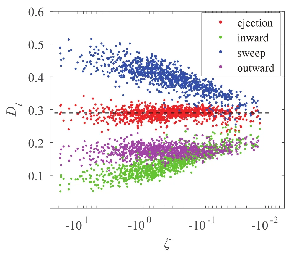
Fig.9.Time fraction of each quadrant Dias a function of the stability parameter.The dotted line represents the mean value(0.29)of the time fraction of the ejections for ζ< −0.02.The value of Diis calculated by dividing the number of T′in the respective quadrants by the total sample number.

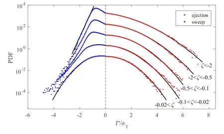
Fig.10.PDF components of ejection and sweep motions under different unstable conditions.For clarity,dots are shifted up:1 unit for−0.1< ζ< −0.02;2 units for−0.5< ζ< −0.1;3 units for−2< ζ< −0.5;4 units for ζ< −2.The vertical dashed line represents T′=0.Solid lines are Gaussian and exponential curves(their functions are presented in Table 3).

The PDF of sweeps changes with instability,being Gaussian in near neutral conditions and close to exponential in very unstable conditions(ζ< −2).The change of PDF type indicates that the property of the air mass may change with stability(Effelsberg and Peters,1983).In near-neutral thermal stratification,shear forces play the main role and the shear instabilities occurs locally(Moeng and Sullivan,1994).In this situation, the property of the air mass in sweep motions is similar to that in ejection motions and follows a Gaussian distribution.Whereas,in strongly unstable conditions,which often occur in a convective boundary layer,downdraughts with cold air from greater height may invade the surface layer(Tillman,1972;Young,1988;Graf et al.,2010).Cold air from high altitude differs from that in the surface layer and may cause the non-Gaussian behavior of sweeps.Some researchers have reported that this “high altitude”may reach the top of the boundary layer.For example,Graf et al.(2010)pointed out that the lowest temperature in the entire boundary layer strongly affects the turbulent PDF,and Mahrt(1991)connected skewness with entrainment processes.These processes may also be the reasons that the skewness and kurtosis of temperature show scatter under the MOST framework,as shown in Fig.5.Therefore,to analyze how such cold air influences the left tail of the PDF,more information on temperature in the mixed layer is needed.

Table 3.Fitted parameters of PDF components of ejections and sweeps under different unstable conditions using Gaussian and exponential functions in Fig.10.

4.Summary and conclusions

The high-order statistics of temperature fluctuations are of great significance for the parameterization schemes in modeling and for basic theory of atmospheric turbulence.Observational data over flat and uniform grassland are used to study the skewness and kurtosis of temperature under the framework of MOST.The temperature skewness and kurtosis generally follow the similarity theory with slight scatter.When the thermal stratification is close to neutral,the temperature follows a near Gaussian distribution.As the instability becomes larger,both the skewness and kurtosis increase and approach constant values(1.5 for skewness and 5.3 for kurtosis)in very unstable conditions(ζ< −2).Similarity functions of skewness and kurtosis derived directly from higherorder moment similarity functions show considerable deviations compared with observation.Therefore,we present new forms of similarity functions of skewness and kurtosis.In the unstable condition,the relationship between skewness and the stability parameter follows S=−7.1ζ/(1−4.8ζ),and that between kurtosis and the stability parameter follows K=(3+9.5ζ)/(1+1.8ζ2).

The fine structure of the temperature PDF under different stratifications is also analyzed,using the quadrant analysis technique.Results indicate a close relationship between the PDF and ejections and sweeps.In unstable conditions,sweeps control the left tail,while ejections control the right tail,of the PDF.The difference in statistical characteristics between ejections and sweeps results in the asymmetry of the PDF.Increasing the duration of sweeps causes the peak of the PDF to become larger with instability.Re fined analysis of the temperature PDF reveals that the temperature fluctuations in the ejection movements obey a Gaussian distribution and that the PDF of temperature in the sweep movements varies with the stability.It should be noted that both“statistical factors”,such as stationarity(Liang et al.,2014;Babi´c et al.,2015),and “process factors”,such as advection and entrainment(Mahrt,1991;De Bruin et al.,1999;Moene et al.,2006;Van De Boer et al.,2014),will cause departure from MOST.How to distinguish and quantify these factors is an interesting topic and needs more combined observations of the surface layer and mixed layer.

Acknowledgements.This research was supported by the National Key Research and Development Program of China(2017YFC0209605)and the National Natural Science Foundation of China(Grant Nos.11472272,41605010 and 41675012).