Assimilation of Sea Surface Temperature in a Global Hybrid Coordinate Ocean Model

Yueliang CHEN,Changxiang YAN,and Jiang ZHU

1International Center for Climate and Environment Sciences,Institute of Atmospheric Physics,Chinese Academy of Sciences,Beijing 100029,China

2University of Chinese Academy of Sciences,Beijing 100049,China

3State Key Laboratory of Acoustics,Institute of Acoustics,Chinese Academy of Sciences,Beijing 100190,China

ABSTRACT The Hybrid Coordinate Ocean Model(HYCOM)uses different vertical coordinate choices in different regions.In HYCOM,the prognostic variables include not only the seawater temperature,salinity and current fields,but also the layer thickness.All prognostic variables are usually adjusted in the assimilation when multivariate data assimilation methods are used to assimilate sea surface temperature(SST).This paper investigates the effects of SST assimilation in a global HYCOM model using the Ensemble Optimal Interpolation multivariate assimilation method.Three assimilation experiments are conducted from 2006–08.In the first experiment,all model variables are adjusted during the assimilation process.In the other two experiments,the temperature alone is adjusted in the entire water column and in the mixed layer.For comparison,a control experiment without assimilation is also conducted.The three assimilation experiments yield notable SST improvements over the results of the control experiment.Additionally,the experiments in which all variables are adjusted and the temperature alone in all model layers is adjusted,produce significant negative effects on the subsurface temperature.Also,they yield negative effects on the subsurface salinity because it is associated with temperature and layer thickness.The experiment adjusting the temperature alone in the mixed layer yields positive effects and outperforms the other experiments.The heat content in the upper 300 m and 300–700 m layers further suggests that it yields the best performance among the experiments.

Key words:ensemble optimal interpolation,multivariate data assimilation,sea surface temperature,ocean heat content.

1.Introduction

The sea surface temperature(SST)is very important for ocean forecasting,global climate monitoring and other marine applications(Gill,1983;Fu et al.,1986;Picaut and Delcroix,1995;Durand et al.,2003;Mayer et al.,2016).Accurate representation of SST in numerical ocean models can improve climate and weather prediction systems.Although considerable effort has been made(Vialard et al.,2001,2002;Zeng and Beljaars,2005;Large and Caron,2015;Giglio et al.,2017;Wang et al.,2017)to improve model performance,numerical ocean models still have difficulties in properly simulating SST due to approximate representation of physical processes,imperfect resolution,and inaccurate atmospheric boundary conditions(Griffies et al.,2000;Griffies and Adcroft,2008).With the increased availability of remotely sensed observations,data assimilation,which optimally combines observations with numerical models,has proved to be a powerful tool to reduce uncertainties(Ezer and Mellor,1994,1997;Aikman et al.,1996;Horton et al.,1997;Behringer et al.,1998;Carton et al.,2000;Kelley et al.,2002;Tian et al.,2014).

Remotely sensed SST observations have near-global coverage but only provide sea surface information.Various data assimilation schemes have been developed to assimilate SST observations.The most straightforward scheme is to directly insert them into an ocean model(Rosati et al.,1997;Syu and Neelin,2000;Tang and Hsieh,2003;Twigt et al.,2007).Such a scheme can lead to an imbalance between the thermal and dynamical fields(Tang et al.,2004).To alleviate this imbalance,some schemes either directly project SST into the subsurface based on the relationship between the SST and the subsurface temperature, or assimilate proxy data estimated by the statistical relationship between temperatures at adjacent depths using temperature analyses at shallow levels(Tangand Kleeman,2002;Tang et al.,2004;Shu et al.,2009).With progress in data assimilation techniques,multivariate assim-ilation schemes[e.g.,three-dimensional variational assimilation(Han et al.,2013;Fujii et al.,2015),Singular Evolutive Extended Kalman(Testut et al.,2003),Ensemble Optimal Interpolation(EnOI)(Oke et al.,2008;Yan et al.,2015;Ji et al.,2015),Ensemble Kalman Filter(Seo et al.,2010;Sakov et al.,2012;Xie et al.,2017),Analysis Correction Scheme(O’Dea et al.,2012;Martin et al.,2007;Storkey et al.,2010)]have been used to assimilate SST.However,in most of the literature listed above,multivariate assimilation methods were used to assimilate SST observations along with vertical profiles and altimetry measurements.Few works have focused on the exclusive assimilation of SST.Additionally,unlike common ocean models,the Hybrid Coordinate Ocean Model(HYCOM)includes a layer thickness variable,as well as the temperature,salinity and horizontal currents.In this paper,we investigate the impact of SST assimilation on the subsurface temperature and salinity in a global HYCOM simulation using the EnOI multivariate method.

This paper is organized as follows:The model,observations and assimilation method are brie fly described in section 2.The design and evaluation of the experiments are presented in section 3.The conclusions are presented in section 4.

2.Model and assimilation

2.1.Model

Version 2.2 of HYCOM,which was developed at the University of Miami(Bleck,2002;Chassignet et al.,2003)and upgraded by the Nansen Environmental and Remote Sensing Center in Norway(Bertino et al.,2008;Sakov et al.,2012),is used in this study.The model uses hybrid vertical coordinates;thus,it can smoothly transition among three types of vertical coordinates in different regions.It is isopycnal in the open,stratified ocean,smoothly reverts to a terrain-following coordinate in shallow coastal regions,and transitions to a zlevel coordinate in the mixed layer or unstratified ocean.The hybrid coordinates are helpful to properly retain water mass characteristics and represent ocean thermodynamic processes and ocean flow.

The model has a global coverage(see Fig.1),with the horizontal model grid created by a conformal mapping in which the North Pole is moved into Eurasia(Bentsen et al.,1999).The grid has 1800×1200 horizontal grid points with approximately 17–25 km grid spacing.The model has 30 hybrid layers,with reference potential densities of 10.1,10.2,10.3,10.4,10.5,30.83,31.11,31.73,32.19,32.68,33.36,33.87,34.22,34.66,35.07,35.50,35.83,36.07,36.25,36.38,36.47,36.65,36.82,36.93,37.01,37.08,37.15,37.19,37.21 and 37.24.The top five layers are low to remain z-level coordinates with a minimum thickness of 3 m.The model bathymetry is interpolated from ETOPO5 gridded data from the National Geophysical Data Center database(NOAA,1988).The mixed layer scheme uses the K-Pro file Parameter(Large et al.,1994,1997).

The model is initialized using version 3.0 of the Polar Science Center Hydrographic Climatology(Steele et al.,2001)and driven by the monthly climatology forcing fields for a 100-yr spin-up.Then,it is forced by the 6-h air temperature,winds,mean sea level pressure,dewpoint temperature,total cloud cover,and precipitation from ERA-Interim(Dee et al.,2011)from 1981 to 2006.The model fields are relaxed toward the same monthly climatology with an e-folding time of 30 days at the sea surface and lateral boundary.

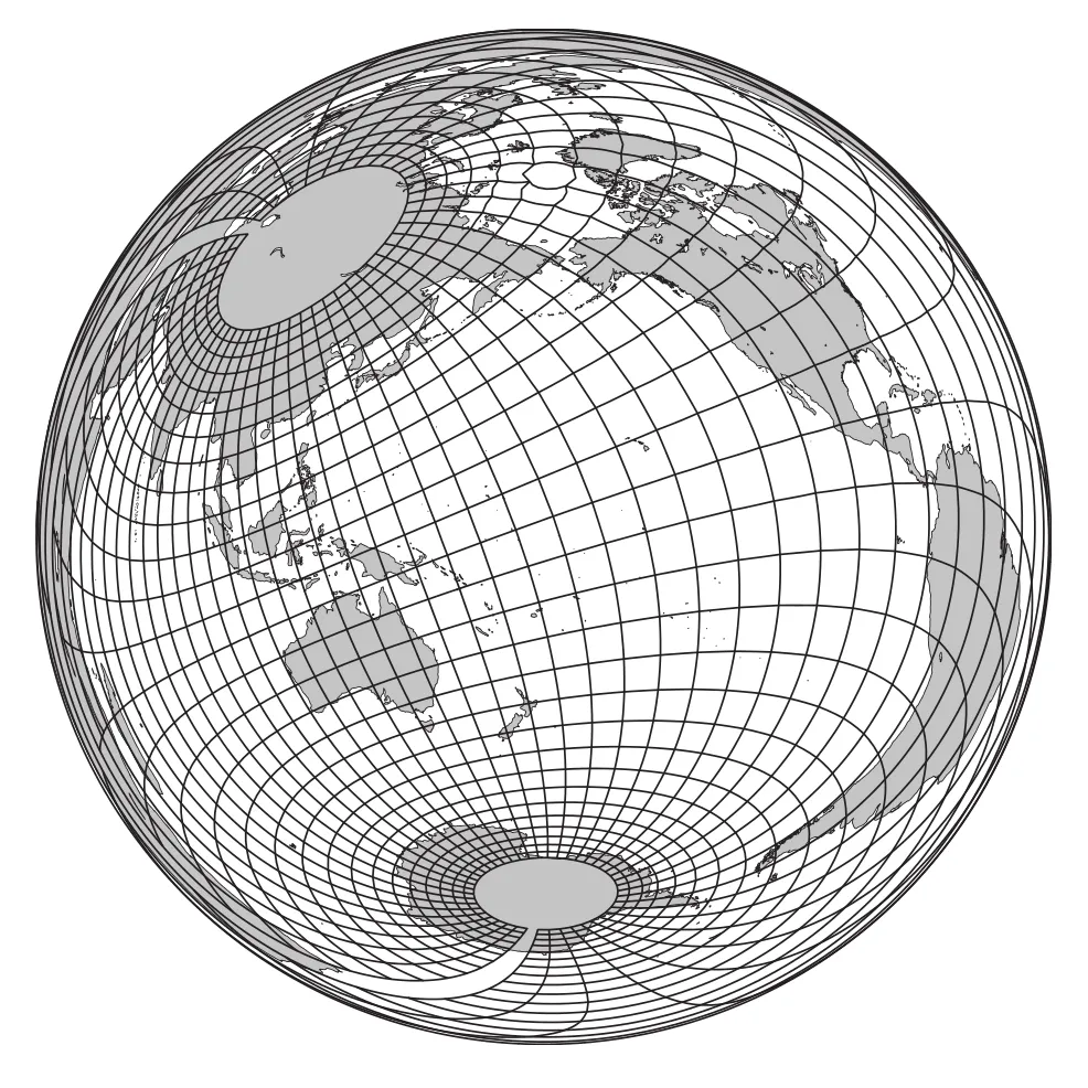
Fig.1.Grid layout of the model.The meshes are drawn every 20 grids for the model domain.

2.2.Observations

The SST data from OISSTv2(Reynolds et al.,2007)are used for assimilation since it is often not practical to use actual observations in as raw a form as possible.The analysis is generated using optimum interpolation.The AVHRR infrared satellite and AMSR satellite data,as well as in-situ observations from ships and buoys obtained from ICOADS,are used in the analysis.Moreover,the analysis also includes a large-scale adjustment of satellite biases with respect to insitu observations and fills in the missing satellite data gaps with different smoothing.It is available from 1981 to present at a horizontal resolution of 0.25°and a temporal resolution of one day.The observational errors are taken from the dataset provider.

2.3.Assimilation method

An ensemble-based method,EnOI(Evensen,2003),is used in this paper.The analysis equation is given as

The background error covariance matrixis de fined as

To reduce the sampling error and avoid false long distance correlations,the background error covariance matrixis localized by the correlation function L.Every element of L is defined by the quasi-Gaussian function of Gaspari and Cohn(1999).The horizontal localization length scale is uniformly 400 km.

3.Results

EnOI is a multivariate assimilation method.That means all model variables may be adjusted by the assimilation of the observations of one variable.In HYCOM,the model variables contain not only the traditional temperature,salinity and current velocities,but also layer thicknesses.In this section,we investigate the impact of SST assimilation in HYCOM via EnOI.

3.1.Experiment settings

To examine the impacts of SST assimilation,we carry out four experiments for the period 2006–08.

Similar to previous studies using the multivariate method(Oke et al.,2008;Sakov et al.,2012;Yan et al.,2015;Seo et al.,2010;Ji et al.,2015),the first experiment modifies all model variables in the assimilation(hereafter called Assim MultiVar).That means that the analysis update is carried out for all variables.The second experiment modifies only the three-dimensional temperature in the entire water column(hereafter called AssimTonly).The analysis update is done for the temperature alone in the entire water column.The third experiment modifies only the temperature in the mixed layer(hereafter called AssimTmxl).In AssimTmxl,a function of depth Lvis used and is expressed as

where hmxldenotes the mixed layer depth(MLD)and z denotes the depth.In fact,the function Lvis equivalent to a vertical localization.At z=hmxl,Lvdrops to a minimum(non-zero value),which indicates Lvis discontinuous.Since the correlation between SST and subsurface temperature estimated by the ensemble gradually decreases with depth in the mixed layer,it is relatively lowatz=hmxl.Both the low correlation and Lvminimum make the analysis increment so small that the effect due to the discontinuity may be neglected.The corresponding analysis equation is given by

In the three assimilation experiments,only the OISSTv2 data are assimilated,with a seven-day assimilation cycle.

As a comparison,a control experiment without any assimilation is also performed(hereafter called CNTL).Table 1 details the design of the experiment.Since the sea-ice model is being tuned,we focus on the region between 60°S and 60°N in this paper.

3.2.Impacts on SST

ICOADS(Freeman et al.,2017)contains surface marine observations from ships,buoys and other platform types.It is used to validate the impacts of the assimilation on the SST.Although ICODAS is not independent,it is a set of direct measurements rather than an analysis,and thus has gone through less processing.Moreover,it is only a small fraction of the data used to generate the OISSTv2 analysis.To assess the assimilation performance,the root-mean-square error(RMSE)is used as an evaluation metric.The RMSE is de fined as

where e denotes the simulated results from different experiments,o denotes the observations,and n is the number ofvalues in the data.In addition,we also de fine the impact of assimilation(IOA)as

Table 1.Experiment design.

where RMSEAssimand RMSECNTLrepresent the RMSEs of the assimilation experiments and the control experiment relative to observations,respectively.The IOA is the percentage reduction in RMSE.When the IOA is positive,the RMSE from the assimilation experiments is reduced,and the assimilation provides a better ocean state than the control experiment.The larger the positive IOA,the greater the improvement due to assimilation.

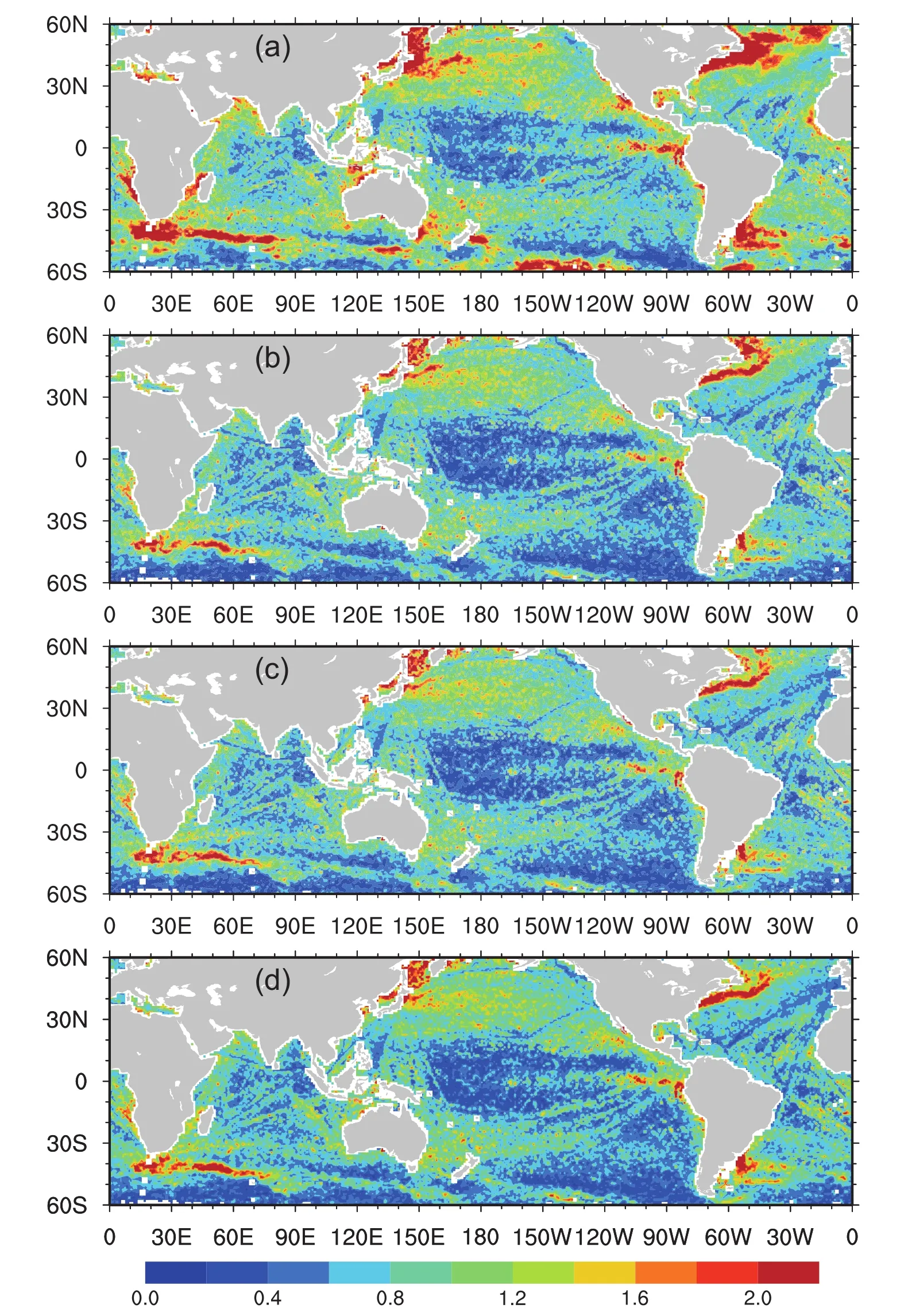
Fig.2.SST RMSEs(units: °C)from different experiments:(a)CNTL;(b)Assim MultiVar;(c)Assim Tonly;(d)AssimTmxl.

Figure 2 shows the spatial distribution of SST RMSEs against ICOADS from the different experiments.The experiment without any assimilation exhibits large RMSEs in coastal regions and regions with abundant eddies(e.g.,the Kuroshio Extension,Gulf Stream system,Agulhas Current,Brazil and Malvinas Con fluence region in the southwestern Atlantic,and Antarctic Circumpolar Current).It is evident that the RMSEs of the three assimilation experiments are greatly reduced in the global ocean.Visually,the experiment AssimMultiVar,which adjusts all variables,exhibits large RMSEs in the Kuroshio Extension and Labrador Sea north of Newfoundland compared with the RMSEs of AssimTonly and AssimTmxl,which adjust only temperature.

To further verify the performance of the assimilation,the global ocean is divided into the Pacific,Atlantic and Indian oceans.Moreover,the IOA of SST is calculated for different regions(Table 2).It is clear that the IOA of the three assimilation experiments is greater than 25%in the global ocean,which indicates that the SST assimilation has a prominent impact(approximately 25%reduction in RMSE)on the SST.The IOA in AssimMultiVar is basically smallest,as shown in Fig.2.This result implies that AssimMultiVar,in which all variables are adjusted,produces the smallest improvement among the assimilation experiments.In the global ocean,the IOA of AssimTonly is slightly larger than that of AssimT-mxl.The difference is observed in the Indian Ocean,where the IOA is 22.57 for AssimTonly and 21.35 for AssimTmxl.In the Agulhas Current and Antarctic Circumpolar Currentregions with numerous eddies,the reduction in RMSE produced by AssimTmxl is less than done by AssimTonly(Fig.2).Of the different ocean basins,the reduction in RMSE is most remarkable in the Atlantic Ocean(greater than 30%),while it is approximately 21%and 18%in the Indian Ocean and Pacific Ocean respectively.In the Atlantic Ocean,the results of AssimTonly are slightly better than those of AssimT-mxl.In the Gulf Stream and Brazil and Malvinas Con fluence regions,AssimTonly produces lower RMSE than AssimTmxl(Fig.2).In the Pacific,AssimTmxl slightly outperforms AssimTonly.

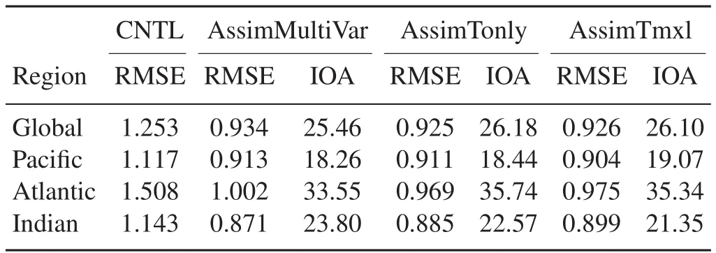
Table 2.Comparison of RMSE(units:°C)and IOA for SST in different experiments and different regions of the global ocean.

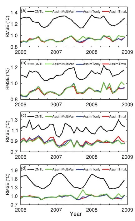
Fig.3.Time series of SST RMSEs(units: °C)in different regions and for different experiments:(a)Global Ocean;(b)Pacific Ocean;(c)Indian Ocean;(d)Atlantic Ocean.

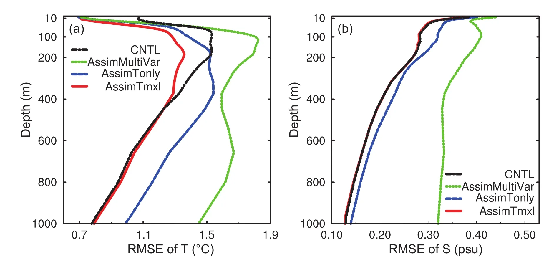
Fig.4.Vertical distribution of the RMSEs of global(a)temperature(units:°C)and(b)salinity(units:psu)for different experiments over the period 2006–08.

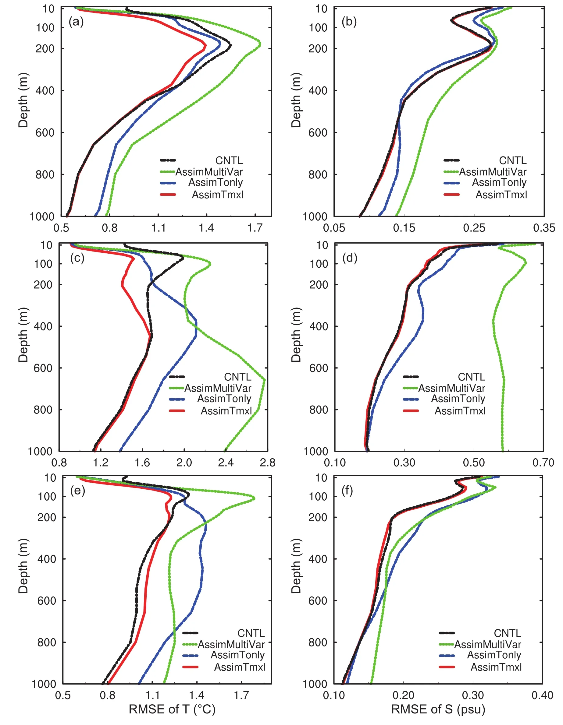
Fig.5.Vertical distribution of the RMSEs of(a,c,e)temperature(units:°C)and(b,d,f)salinity(units:psu)for different ocean basins and different experiments:(a,b)Pacific Ocean,(c,d)Atlantic Ocean;(e,f)Indian Ocean.

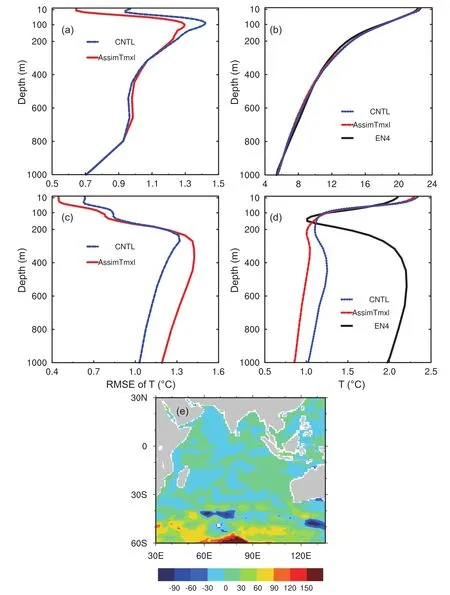
Fig.6.(a,c)RMSEs of temperature(units:°C)and(b,d)area-averaged temperature pro files(units:°C)for different experiments and different regions:(a,b)Indian Ocean north of 50°S;(c,d)Indian Ocean south of 50°S.(e)Difference in MLD between CNTL and EN4.2.0 in the Indian Ocean.

In Fig.3,the time series of SST RMSEs are shown for various experiments and regions.For the global ocean,the RMSEs of the control experiment are approximately 1.3°C during the entire simulation period,and the RMSEs of the three assimilation experiments are reduced to less than 1°C(Fig.3a).AssimMultiVar exhibits a larger RMSE than AssimTonly and AssimTmxl in the second halves of 2007 and 2008(Fig.3a).The relatively large RMSE of AssimMultiVar is mainly in the Atlantic Ocean(Fig.3d).Also,the RMSE of SST varies in different regions.Specifically,the highest RMSE can be observed in the Atlantic Ocean,and the RMSE in the Pacific Ocean is slightly lower than that in the Indian Ocean.Moreover,the three assimilation experiments exhibit different improvements in different regions.In the Pacific Ocean,the three assimilation experiments exhibit similar improvements,except AssimMultiVar at the end of 2008.In the Indian Ocean,AssimTmxl exhibits a slightly larger RMSE than both AssimMultiVar and AssimTonly,as shown in Table 2.In the Atlantic Ocean,AssimMultiVar displays higher RMSEs in the second half of both 2007 and 2008 compared to those of AssimTonly and AssimTmxl.Overall,the three assimilation experiments yield pronounced SST improvements over the control experiment in different regions,and both AssimTonly and AssimTmxl outperform AssimMultiVar.

3.3. Impacts on subsurface temperature and salinity

SST observations provide sea surface information.Therefore,it is natural that the assimilation process improves the modeled SST.Whether or not the subsurface thermohaline structure is improved is investigated in this section.As independent observations,the monthly temperature and salinity objective analyses from EN4.2.0(Good et al.,2013)are used to validate the impacts of SST assimilation on the subsurface temperature and salinity.The bias corrections from Gouretski and Reseghetti(2010)are applied in the objective analyses.The World Ocean Database 2013,Global Temperature and Salinity Pro file Project,Array for real-time geostrophic oceanography,and Arctic Synoptic Basin-wide Observations project datasets are used to create EN4.2.0.

Figure 4 shows the vertical distribution of the RMSEs of global temperature and salinity.For global temperature,AssimMultiVar,which adjusts all model variables,produces an improvement over the control experiment in the upper 50 m and a significant decline below 50 m.This result is potentially associated with an improper correlation between the layer thickness and SST.A small change in the layer thickness can induce a large change in the temperature,especially in the thermocline region.AssimTonly,which adjusts only the temperature in the entire water column,yields an improvement in the upper 170 m and a decline below 170 m.The improvement of AssimTonly reaches a greater depth than that of AssimMultiVar.Additionally,the decline is likely associated with an improper correlation between the subsurface temperature and the SST described by the ensemble members.AssimTmxl,which adjusts only temperature in the mixed layer,exhibits the best performance.This result implies that the SST assimilation affects not only the SST but also the subsurface temperature in the upper 400 m.For global salinity,AssimMultiVar exhibits the worst performance and the largest RMSE.Additionally,AssimTonly has a negative impact,and the results of AssimTmxl are similar to those of the control experiment.The salinity is associated with the layer thickness and temperature in the model.The negative impact is partly attributable to the layer thickness and partly to the temperature.

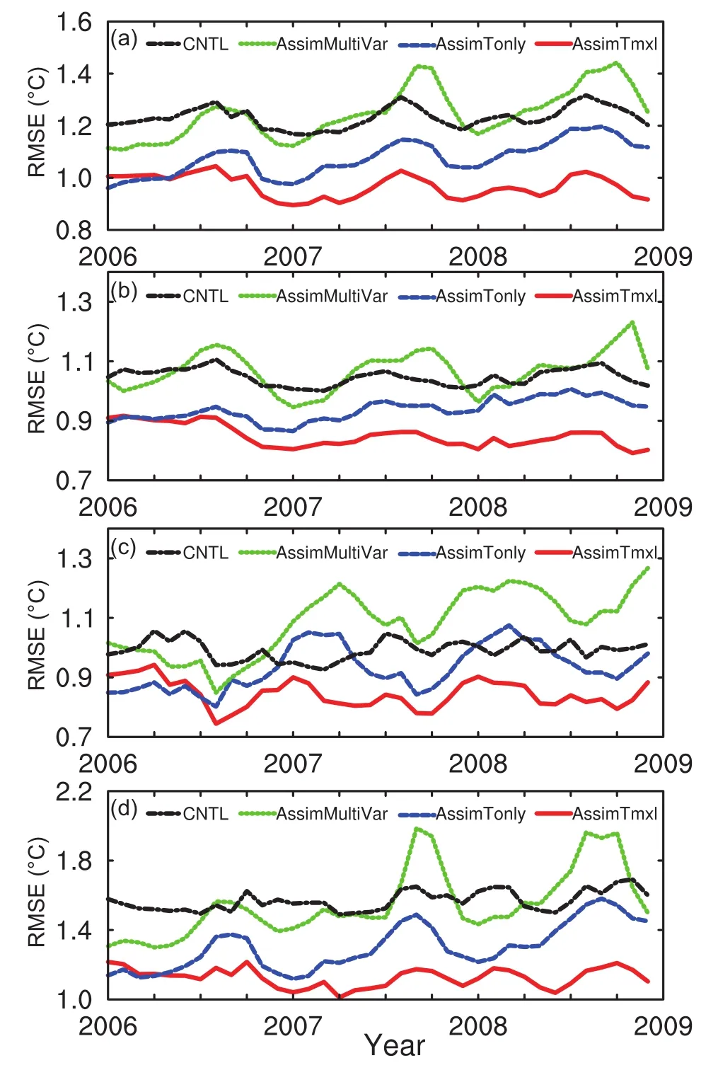
Fig.7.RMSEs of HC300(units: °C)in different regions and for different experiments:(a)Global Ocean;(b)Pacific Ocean;(c)Indian Ocean;(d)Atlantic Ocean.

In different ocean basins,the vertical distribution of the RMSE of temperature and salinity is different(Fig.5).AssimMultiVar performs worst in the three ocean basins,with a temperature improvement in only the upper 50 m and a salinity deterioration in the entire water column in the three ocean basins.Notably,AssimMultiVar yields the largest RMSEs in the Atlantic Ocean,especially below 500 m,which contributes considerably to the global RMSE.For temperature,AssimTonly produces an improvement above the thermocline and a decline below the thermocline in the three ocean basins.This result indicates that the correlation between the subsurface temperature below the thermocline and the SST is possibly poor.Additionally,AssimTonly has negative impacts on salinity in the three ocean basins.AssimTmxl exhibits the best performance in the three ocean basins.In the Indian Ocean,it has a slightly larger temperature RMSE compared with that of the control experiment below 250 m.This difference is mainly from the zonal band of 60°S–50°S in the Indian Ocean(Fig.6c).For temperature,the RMSE of AssimTmxl is similar to that of CNTL in the Indian ocean north of 50°S(Fig.6a),while it is notably larger than that of CNTL south of 50°S(Fig.6c).The large difference is probably associated with the temperature inversion(Fig.6d)and an improperMLDsimulatedbythemodel(Fig.6e).SinceAssimT-mxl adjusts only the temperature in the mixed layer,a deep MLD leads to the propagation of SST observation information to a greater depth in the assimilation process,resulting in a large RMSE.

3.4.Impacts on the heat content

The heat content represents the heat stored in the ocean and is an important factor determining subsurface temperature changes.The impacts of three different assimilation experiments on the heat content are investigated in this section.

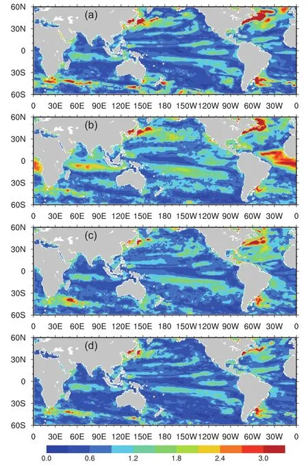
Fig.8.RMSEs of HC300(units: °C)for different experiments over 2006–08:(a)CNTL;(b)AssimMultiVar;(c)AssimTonly;(d)AssimTmxl.

Generally,the ocean heat content in the upper 300 m(called HC300)is de fined as the temperature averaged over 0–300 m.Similarly,HC300–700 represents the temperature averaged over 300–700 m.Figure 7 shows the time series of HC300 RMSEs relative to the EN4.2.0 analyses for different ocean basins.The RMSE over the global ocean produced by AssimMultiVar is smaller than that of CNTL before 2007 and increases with time after 2007(Fig.7a).Similarly,the RMSE produced by AssimTonly also exhibits an increasing trend,although it is lower than that of CNTL from 2006–08.In fact,there is not an increasing trend in the RMSE of CNTL.Thus,the error induced by adjusting all model variables or only temperature in the entire water column in the assimilation is gradually amplified with time.The RMSE of AssimTmxl is the lowest,and its evolution with time is the same as that of CNTL.

In the three ocean basins,both AssimMultiVar and AssimTonly exhibit an increasing RMSE with time,which leads to a rising trend in the RMSE over the global ocean.Additionally,AssimMultiVar produces the largest RMSE compared with those of other experiments in the three ocean basins.In the Indian and Atlantic oceans(Figs.7c and d),the RMSE of AssimMultiVar is much greater than that of CNTL.Additionally,the RMSE of AssimTonly gradually approaches that of CNTL with time,although it is lower in the Pacific and Atlantic oceans(Figs.7b and d).In the Indian Ocean,the RMSE of AssimTonly is slightly higher compared with that of CNTL in some periods(Fig.7c).AssimTmxl performs best,with the lowest RMSEs in the three ocean basins.

The spatial distribution of the RMSE of HC300(Fig.8a)is similar to the RMSE of SST for CNTL.Large RMSEs mainly occur in regions with abundant eddies or strong western boundary currents or Antarctic Circumpolar Current.Additionally,the large RMSEs can be observed in the equatorial Indian and Pacific oceans.Compared with CNTL,Assim-MultiVar significantly increases the RMSE,especially in the equatorial Indian and Atlantic oceans(Fig.8b).This result implies that the large RMSE of HC300 in the model simulation contributes to an improper relationship between the variables and the SST,which leads to the poor performance of AssimMultiVar.AssimTonly reduces the RMSE in the global ocean,except in the northern Atlantic south of 30°N(Fig.8c).AssimTmxl decreases the RMSE in the global ocean(Fig.8d).

For the ocean heat content in the upper 300–700 m of the global ocean(Fig.9a),both AssimMultiVar and AssimTonly yield much larger RMSEs than CNTL.Similar to HC300,the RMSE of HC300–700 also increases with time.However,the growth is much faster.This result indicates that the relationship between the SST and the variables of the subsurface estimated by the ensemble is not reasonable.AssimTmxl exhibits a slight improvement over CNTL,potentially because the temperature below 300 m is adjusted by the model dynamics and thermodynamics rather than by the assimilation.In the Pacific and Atlantic oceans,the evolution of the RMSE(Figs.9b and d)is similar to that of the global ocean for all experiments.However,it is different in the Indian Ocean.AssimTonly,instead of AssimMultiVar,exhibits the largest RMSE in the Indian Ocean,as shown in Fig.5e.Moreover,the RMSE of AssimTmxl is slightly greater than that of CNTL(Fig.9c).As noted above,this difference is probably induced by an inaccurately modeled deep mixed layer and a temperature inversion.

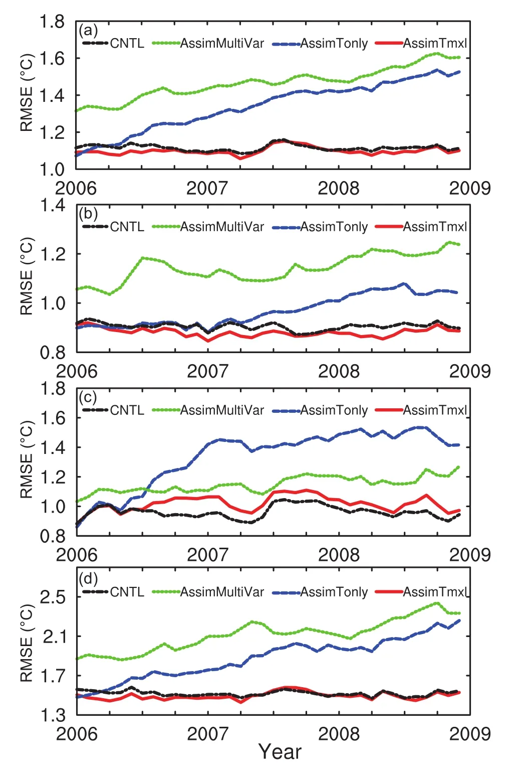
Fig.9.RMSEs of HC300–700(units: °C)in different oceans and for different experiments:(a)Global Ocean;(b)Pacific Ocean;(c)Indian Ocean;(d)Atlantic Ocean.

The distribution of the subsurface temperature error below 300 m(see Fig.10)is different from that in the upper 300 m(Fig.8).For CNTL,the simulated large RMSE of HC300–700 in the Gulf Stream region extends southward,and the RMSEs in the tropical Indian and Pacific oceans are lower than those of HC300,although the large RMSEs associated with eddies are still present(Fig.10a).For AssimMultiVar,the large RMSE of HC300–700 almost spreads throughout the entire Atlantic Ocean.Moreover,the RMSE is further enhanced compared with that of CNTL in the Indian and Pacific oceans.The RMSE of AssimTonly exhibits a pattern similar to that of CNTL,but is much higher in the large-RMSE regions.This result implies that the large errors simulated by the model may lead to an improper correlation between the SST and the subsurface temperature.Compared with AssimTonly,the large RMSE of AssimMultiVar in the tropical Atlantic Ocean(40°S–20°N)is probably induced by the unreasonable,or potentially non-existent,correlation between the SST and other variables.The RMSE of HC300–700 for AssimTmxl is similar to that for CNTL because the temperature below the mixed layer is not modified by the assimilation.

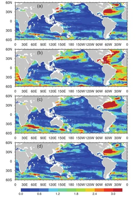
Fig.10.RMSEs of HC300–700(units:°C)for different experiments over 2006–08:(a)CNTL;(b)AssimMultiVar;(c)AssimTonly;(d)AssimTmxl.

4.Conclusions

This study addresses the impact of SST assimilation on the global temperature and salinity simulations of HYCOM with a hybrid vertical coordinate based on the EnOI multivariate assimilation method.Four different runs are carried out for the period 2006–08,of which three are assimilation runs(AssimMultiVar,AssimTonly and AssimTmxl).In AssimMultiVar,all model variables are adjusted.In AssimTonly and AssimTmxl,only the temperature in the entire water column or in the mixed layer is adjusted.A control experiment without any assimilation is also performed for comparison.

The three assimilation runs lead to improved simulations of SST in comparison with the control run without any assim-ilation,as expected.Notably,a reduction(greater than 25%)in RMSE is achieved in the global ocean.The runs that adjust only the temperature alone produce better simulation results than the run that adjusts all model variables.Specifically,in the Atlantic Ocean,a reduction of approximately 35%in RMSE is observed for the runs in which only temperature is modified,and a reduction of approximately 33%is observed for the run in which all variables are modified.

A more stringent validation of the impact of the SST assimilation is carried out by comparing the simulations from the model runs with EN4.2.0 temperature and salinity analyses generated by observations.The vertical distributions of the RMSEs of temperature and salinity show that there is a distinct improvement in temperature,as well as almost no improvement in salinity,as a result of adjusting the temperature alone in the mixed layer in the assimilation.However,there is a negative impact on the temperature at the subsurface and on the salinity throughout the modeled layers when only the temperature in the entire water column or all model variables are adjusted.

The ocean heat content in the upper 300 m of the global ocean is improved by adjusting the temperature in the mixed layer via assimilation.A rising trend in the RMSE of HC300 is observed over time when the temperature in the entire water column is modified or all variables are modified,and the latter yields a much greater RMSE than that of the CNTL experiment without any assimilation.The spatial distribution of the RMSE of HC300 shows that the assimilation in which all variables are adjusted results in large errors in the tropical Atlantic Ocean(15°S–15°N)and further enhances the inherent model errors in the tropical Pacific and Indian oceans.The ocean heat content from 300 m to 700 m reveals the changes in the subsurface temperature induced by the assimilation.Much larger RMSEs than those of the run without assimilation are found when the temperature in all layers is modified or all variables are modified by the assimilation.In addition,the RMSE exhibits an obvious upward trend with time.This result indicates that model performance deteriorates the longer the model integration continues.When the temperature in the mixed layer is modified,the heat content from 300 m to 700 m changes slightly in comparison with that of CNTL.This change is associated with the adjustment of the temperature below the mixed layer by the model dynamics instead of assimilation.The spatial distribution of the ocean heat content from 300 m to 700 m demonstrates that large errors are present almost everywhere in the Atlantic Ocean when all variables are modified in the assimilation.When the temperature alone in the entire water column is modified,the inherent model errors are amplified or extended in the Atlantic and Indian oceans.This result is probably associated with poor correlation between the SST and the subsurface variables due to model errors or spurious correlations.When the temperature alone in the mixed layer is modified,the spatial pattern is similar to that of CNTL.

The results of this study suggest that SST assimilation with only temperature modifications in the mixed layer performs best.AssimTmxl is an experiment in which a special vertical localization technique is used.The technique localizes the influence of SST observations to the mixed layer.For the ensemble-based methods,the ensemble with a finite size approximation to the covariance matrix indicates that the correlations are not real.The spurious correlations can induce variable updates in regions that should not be updated.To eliminate the spurious covariances with distant grid points,the horizontal localization(e.g.,the correlation function L used in this paper)is usually adopted.The performance of AssimTmxl implies that vertical localization is very important,especially for SST assimilation.Moreover,attention should be paid to SST assimilation by ensemble-based multivariate assimilation methods.The ensemble used in the assimilation is usually taken from model outputs.However,model errors can give rise to improper correlation between the SST and other variables,which can lead to the improper adjustment of variables in the assimilation.In particular,when a specific variable is dominant(e.g.,the layer thickness variable in HYCOM),its incorrect adjustment can generate an extensive negative impact on the other variables.

Acknowledgements.This work was supported by the National KeyR&D Program of China(GrantNo.2016YFC1401705),theNational Natural Science Foundation of China(Grant Nos.41176015 and 41776041),the Chinese Academy of Sciences Project“Western Pacific Ocean System:Structure,Dynamics and Consequences”(Grant No.XDA11010203),the Program(Grant No.315030401),and the State Key Laboratory of Tropical Oceanography,South China Sea Institute of Oceanology Chinese Academy of Sciences(Project No.LTO1501).The work was carried out at the National Supercomputer Center in Tianjin,and the calculations were performed on Tian He-1.