Optimal Scheduling of Air Conditioners for Energy Efficiency

K. Venkatesan and Uppu Ramachandraiah

Abstract—Energy saving is one of the most important research hotspots, by which operational expenditure and CO2 emission can be reduced. Optimal cooling capacity scheduling in addition to temperature control can improve energy efficiency. The main contribution of this work is modeling the telecommunication building for the fabric cooling load to schedule the operation of air conditioners. The time series data of the fabric cooling load of the building envelope is taken by simulation by using Energy Plus,Building Control Virtual Test Bed (BCVTB), and Matlab. This pre-computed data and other internal thermal loads are used for scheduling in air conditioners. Energy savings obtained for the whole year are about 4% to 6% by simulation and the field study,respectively.

1. Introduction

Energy conservation and peak demand reduction are the major requirements for reducing CO2emission and maximizing utilization of energy sources[1]. The air conditioners are designed to continue working throughout the year based on the peak thermal. The surfaces heat is absorbed by building fabric,such as walls and floors roof. The infiltration heat varies throughout the year due to the varying climate. Computation of the thermal load of the building fabric in a climate responsive way is one of the challenges for adapting the cooling capacity.Recent research survey indicates that atmospheric temperature has been used for reducing the cooling capacity. Some research survey uses the Kalman filter or the rules based control. This research aims to use software computation of the building fabric thermal load for optimal scheduling of air conditioners.

For small capacity installations, it is common to use a group of direct expansion type air conditioners, such as precision air conditioners (PAC), package type air conditioners,or split air conditioners to share the thermal load. The environmental requirement for telecommunication equipment room is: Temperature (23±3) °C and relative humidity RH=(45±15)%. Normally a cooling system consists ofN+1 air conditioners with equal capacity[2], whereNrepresents the number of air conditioners installed to cater the peak summer load and 1 represents the standby air conditioner. The capacity of the individual air conditioner multiplying the numberNgives the peak cooling capacity. The capacity of theseNair conditioners is arrived based on the peak heat load during summer by taking the hottest temperature of the day[3]. The cool air distribution method is shown in Fig. 1. PAC working in the technology room operates round the clock with a dead band as the set point.

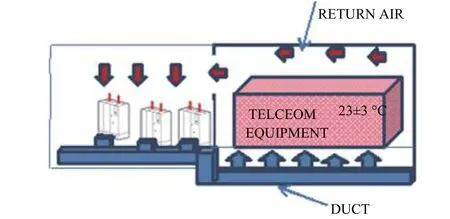
Fig. 1. Telecom equipment air conditioner system.

The operation of this system can be considered as a group of thermostatically controlled loads. Their operations mainly rely on the room temperature. How to best adapt these air conditioners automatically throughout the year for the changing thermal load is the problem of interest.

1.1 Need for Capacity Reduction

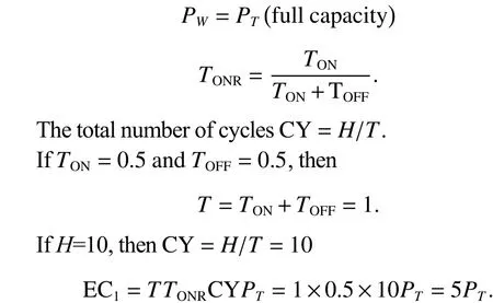
LetITbe the total thermal load at the given control time step,PTbe the total cooling output ofNair conditioners, andPwbe the cooling output of working air conditioners. And letTONbe the ON time per cycle,TOFFbe the OFF time per cycle, andTbe the total time per cycle of the operation of the group of air conditioners for a cycle. AndHrepresents the observation period and CY is the number of cycles duringH.

Case 1. No Change in Thermal Load

The total thermal load isIT, and

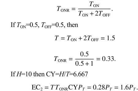
Case 2. Thermal Load Reduced—Air Conditioner Capacity Not Reduced

If the total thermal loadITis reduced toIT/2,TOFF(heating time) becomes double, if the working air conditioners are not reduced, that isPW=PTis continued, it results inTONbecoming half:

Case 3. Thermal Load Reduced—Air Conditioner Capacity Also Reduced

If the total thermal loadITis reduced toIT/2, andPWis also reduced to the half (i.e.PW=PT/2), then both heating time and cooling time gets doubled:

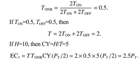
From Case 1, Case 2, and Case 3, it can be observed that,reducing the air conditioner capacity proportional to the thermal load reduces the energy consumption. It is necessary to maintainTON=TOFForTONclose toTOFF. This also reduces the peak energy consumption demand. Accounting the varying thermal load and optimally scheduling these PAC are the problems studied for energy saving. The approach is to deploy cooling load (the number of PAC’s) equal to the thermal load at that instant and it is called as energy balanced air conditioner scheduling (EBACS). M. F.Hanniffet al.[4]classified the scheduling methods of air conditioners into basic techniques, conventional techniques,and advanced techniques. These techniques are applicable to the human comfort air conditioning system. For 24/7 operated buildings (such as telecommunication buildings, data centers,equipment room, etc.), called technology rooms, air conditioning is required round the clock. It is not efficient to increase thermal insulation of the air-conditioned building beyond the certain limit[5], while scheduling the weather condition has to be taken into account[5],[6]. The atmospheric temperature leaded by weather variation has been tracked in [3]and the atmospheric temperature with predictive moving average was described in [4]. In [7] and [8], the low cost web based control and its automation were described, in which, the control is based on room temperature. E. Mohamedet al.[9]used the finite difference method to estimate the cooling load. As stated by S. Armstronget al.[10]the fabric cooling load lags the atmospheric temperature due to the wind speed which plays the major role in infiltration heat and surface convection heat. The parameters, such as the wind parameter, in the conventional thermal load calculation for each step of control further increase the computational complexity. Software based tools,such as Energy Plus, can be used for computing the fabric cooling load by modeling and simulations with the consideration of the fabric construction orientation and climate parameters, such as the atmospheric temperature and wind speed. B. Yuceet al.[11]modeled the building in Energy Plus-Design Builder and obtained the thermal energy consumption and predicted mean vote by using the artificial neural network(ANN). Using these data, the genetic algorithm (GA) rules have been generated for optimization of the heating system.The fabric cooling load of the base transceiver stations (BTS)shelter envelope was modeled in [12] and [13]. In case of telecommunication buildings, normally man power has been engaged to reduce the load: Some air conditioners are switched OFF based on practical experience. This is not an accurate method. In this condition, there is a gap to be addressed for scheduling (changing the capacity of the air conditionersN,N–1,N–2, etc.) the air conditioners based on the thermal load for the whole year. For varying the cooling capacity automatically, the thermal load of the fabric is required along with the internal load. For this the explicit data of thermal load is required, which also helps for monitoring performance of the cooling system. This work is aiming for addressing this research gap. In this paper, a telecommunication building has been modeled by using Energy Plus for obtaining the fabric cooling load. Using this data, simulations based scheduling has been done for the whole year and the field experiment is also conducted. The energy consumption by this method has been compared with the other methods.

1.2 Methodology

Nowadays, most buildings are designed with the building management system (BMS). The thermal load, such as the equipment load, number of persons, and power plug load, can be obtained from BMS. The advanced simulation tools like Energy Plus can estimate the fabric cooling load considering all the climate factors. The exact construction of the building has been modeled in Energy Plus to get the fabric cooling load with the time step of 15 minutes throughout the year. This data can be used in real time by two methods as shown in Fig. 2. The first method uses the simulated data directly in the scheduler for every 15 minutes throughout the year. In this method, the fabric cooling load data obtained from Energy Plus is about 35040 samples for the whole year, which is used in a time synchronized manner throughout the year. The second method uses curve fitting on simulated monthly data over the atmospheric temperature for twelve months. These monthly curve is selected in a time synchronizing manner. Using the curve constants and the atmospheric temperature, the fabric cooling load can be computed for every control step. Fig. 3 shows BMS. Fig. 4 shows the division of thermal load for air conditioners. As mentioned in [11] and [12], it is more efficient to use the fabric cooling load computed with the wind speed and other parameters than only considering the temperature change in the atmosphere[3]. The field study has been conducted in the same building to validate the proposed method. Recently most researchers use Energy Plus for their studies[12]-[18]. With the help of this simulation, setting up the whole year fabric cooling load of the building can be obtained as time series data for real time control or scheduling. The lumped RC model[12],[13],[19]-[22]has been used for the simulation based comparison of energy consumption.

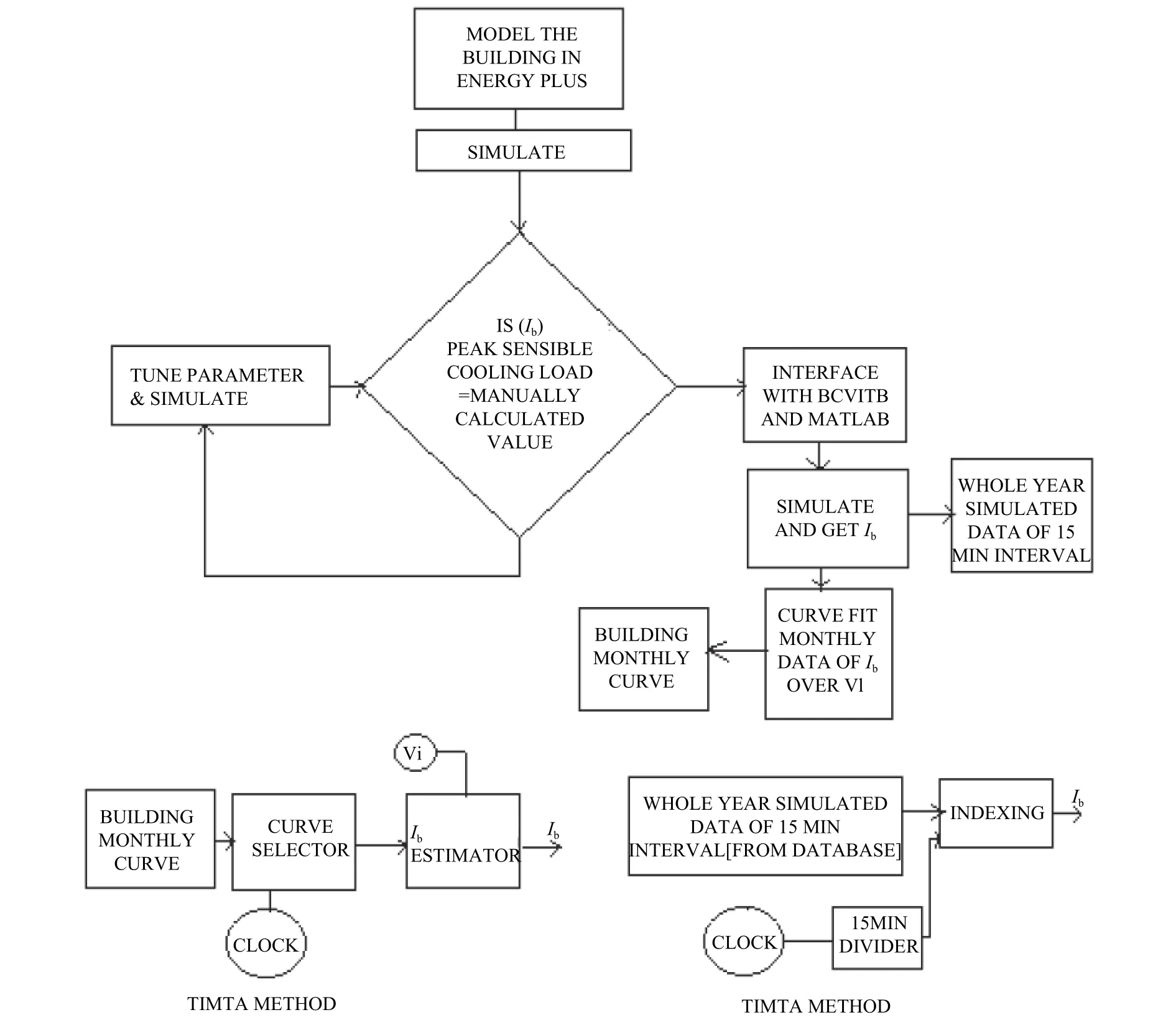
Fig. 2. Methodology of building fabric cooling load measurement.

The rest of the paper is organized as follows. Section 3 describes the building thermal load and modeling in Energy Plus software. Section 4 deals with the RC model. In Section 5 approaches for scheduling the air conditioners have been discussed. Section 6 details the field study and in Section 7 results are discussed.

2. Building under Study

2.1 Building Parameters

A technology room housing telecommunication equipment was chosen for study. The building is in Chennai longitude 13°N and latitude 80.18°E. The details of peak heat load of the building are shown in Fig. 5. These parameters are arrived using the conventional heat load calculation method. The building construction parameters are shown in Table 1. The view of building (modeled in Energy Plus software) in Open Studio software is shown in Fig. 6 and Fig. 7.

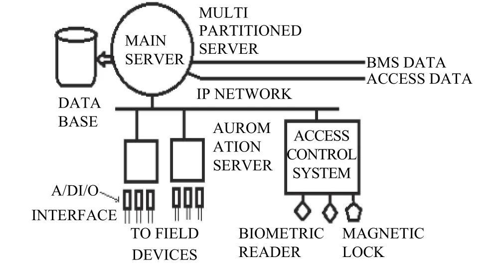
Fig. 3. Typical BMS.

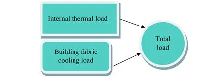
Fig. 4. Thermal load of building for air conditioners.

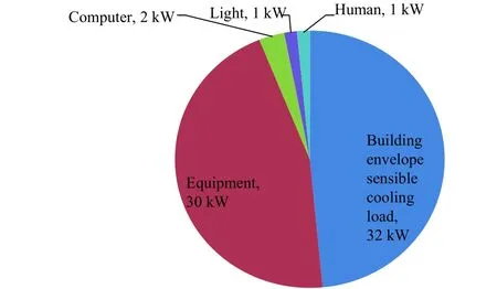
Fig. 5. Building peak heat load.

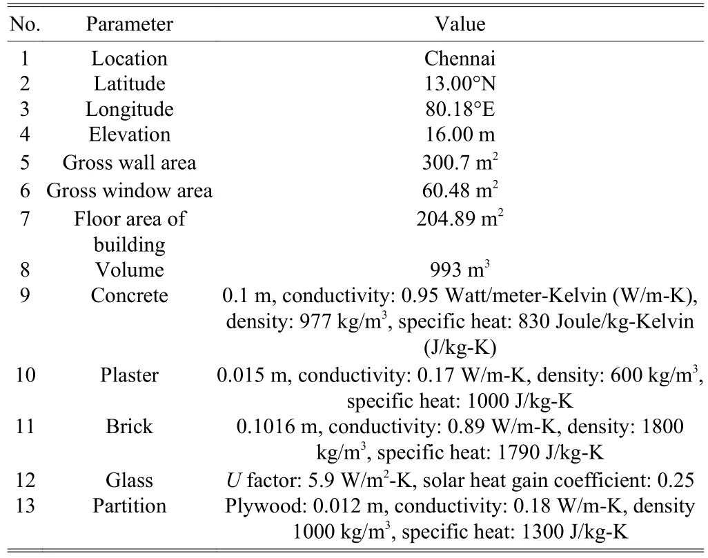
Table 1: Building parameters

Fig. 6. Open studio view of the building modeled in Energy Plus.

Fig. 7. Open studio view of the building modeled in Energy Plus(transparent view).

The building envelope heat load or building fabric cooling load, also called building heat absorption or building envelope sensible cooling load, consist of the heat absorbed by the opaque surfaces, window heat addition, and infiltration heat:

whereIbis the building fabric cooling load in kW,IINFis the infiltration heat,Iwis the window heat addition, andIOPQis the heat absorbed by the opaque surfaces. The peak building fabric cooling loadIbcan be directly obtained from Energy Plus without other software which occurs on the 9th of May.

The selected building has the peak sensible cooling of about 32.24 kW comprising 4.05 kW window heat addition,19.59 kW infiltration heat, 9.127 kW opaque surface conduction,and other heat additions. This value is obtained by the simulation of Energy Plus for the room set point of 23 °C. But this value goes to zero in most of the period during January as shown in Fig. 8. If the capacity is not reduced, it would result in wastage of energy and the room temperature may go below the set value. Hence the capacity reduction is important. It is essential to schedule the air conditioner in an energy balanced manner, i.e. proportional to the thermal load.

Fig. 8. Building fabric cooling load for the month of May and January.

2.2 Measurement of Heat Load

Nowadays it is customary to induct the BMS in the modern telecommunication buildings/data centers. The following internal loads A to E can be obtained from BMS.

A. Heat Load Due to Lighting

The lighting load is nowadays controlled using occupancy sensor. The heat produced by the lights can be obtained using the equation:

whereIIis the lighting load in kW,Soiis the occupancy sensor (1 for occupied and 0 for unoccupied),niis the number of lamps controlled by the sensorSoi,Liis the wattage of individual lamp in kW, andkis the maximum number of sensors. By knowing the occupancy statusSoithe lighting load can be easily calculated and hence the heat produced by the lights. Alternatively theIIcan be obtained by usingwhereVis the supply voltage,Iis the lighting load current, andis the average power factor.

B. Human Heat Load

The number of people present in the room is easily obtained by using the access control system. Using the value of latent heat per person 310 (British Thermal Unit) BTU/Hr and sensible heat 240 BTU/Hr. The heat load of a person works out to 550 BTU/Hr=0.16 kW. The total human heat loadIHcan be obtained asIH=0.16wkW, wherewis the maximum number of people.

C. Power Plug Load

The total power plug loadIPin kW is

whereSpiis the power plug sensor value (0 or 1),Lpiis the power plug load of theith load in kW, andvis the total number of power plug loads. If the power plug load is variable then the same can be obtained by measuring the current to get that the power is similar to light load quoted above.

The power plug such as computer load and any other power plug can be obtained by the sensor of the power plug.Multiplying the wattage, the heat produced by the power plug load can be obtained. The embedded web server based electrical load management has been discussed in [23].

D. Equipment Load

The equipment operates at 50 V DC. Using the rectifier, the 50 V DC is obtained from 415 V AC supply. The equipment heat load is obtained by using

whereVis the voltage,Iis the DC current, andηis the efficiency of the rectifier. The voltageVis normally constant. By measuring the DC currentI, the instantaneous heat generated by the equipment can be calculated.

E. Building Envelope Heat Load: Climate Material Time Modularity (CLIMATMO) Problem with 1) Temperature-Time(TEMTIM) Solution, and 2) Time, Data (TIMTA) Solution

The building fabric cooling load depends not only on the atmospheric temperature, but also varies with the respect to climate, material of the construction of the building and time.In other words, the climate is various with respect to time due to various seasons. Modularity of the building comprises of orientation of the building and volume of the building. This CLIMATIMO problem is simplified by modeling the building envelope in Energy Plus and getting the fabric cooling load for the given set point. Using simulated data, curve fitting can be done as discussed in Section 4. Using curve, atmospheric temperature and time, the building envelope fabric cooling load can be calculated for any instant of time throughout the year.This method is called TEMTIM. The TIMTA method refers to storing the simulated data of fabric cooling load samples in the memory and accessing the same in the time synchronized manner. For the telecom application, the set point is constant round the clock, throughout the year. The building design is fixed and the orientation with respect to the sun is fixed, so the fabric cooling load pattern is taken as fixed (on yearly basis).When there is large deviation in climate data, then this data has to be updated. In case of TEMTIM method, the atmospheric temperature deviation is discussed in detail in subsection 5.3.The TEMTIM method can be used even if there is wide variation in climate data.

The Energy Plus simulation gives building fabric cooling loadIb, one peak value for the whole year. But thisIbvaries throughout the year round the clock. Hence to get the continuous value, the Energy Plus is interfaced with Matlab and Building Control Virtual Test Bed (BCVTB). The Matlab cannot directly communicate with the Energy Plus. The BCVTB acts as the interface between the two software. The Simulink gives a set point value to Energy Plus via BCVTB[12],[13],[15]. For the given room temperature set point, the Energy Pus gives out the building envelope fabric cooling load.The sampling time is 15 minutes for the given simulation period. Fig. 9 shows the data flow diagram. The Ptolemy model[15]is depicted in Fig. 10. By simulation, the building fabric cooling load and other climate parameters are obtained via BCVTB.

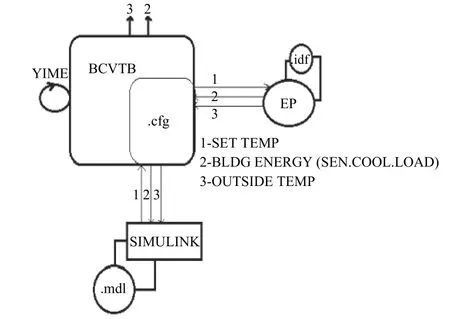
Fig. 9. Data flow diagram for getting building fabric cooling load.

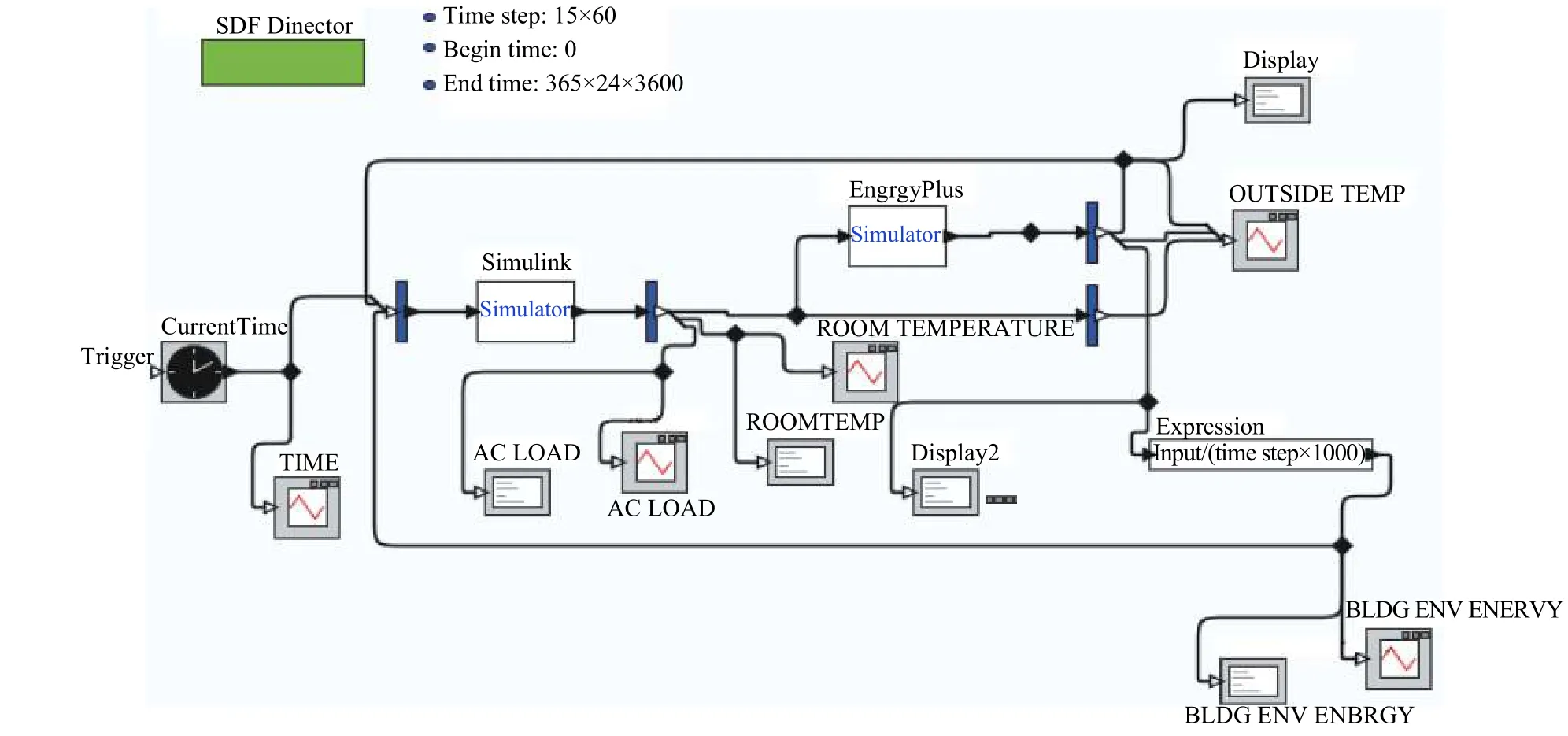
Fig. 10. Ptolemy model.

3. Building RC Model

3.1 Parameters Estimation

For simulation in Simulink, the air conditioners, building envelope thermal load, and equipment load are considered as current sources in kW (using the electrical-thermal anology[12],[20],[21]). The voltage is considered as temperature °C.Since the building is with a huge thermal constant and temperature band for operation, the lumped RC model of the building under study is formulated as shown in Fig. 11. The Simulink contains the building RC model. For each sample of simulation, the air conditioner output, room temperature, and other parameters are obained in BCVTB. To describe the RC model in detail, the paramaters are defined as follows:

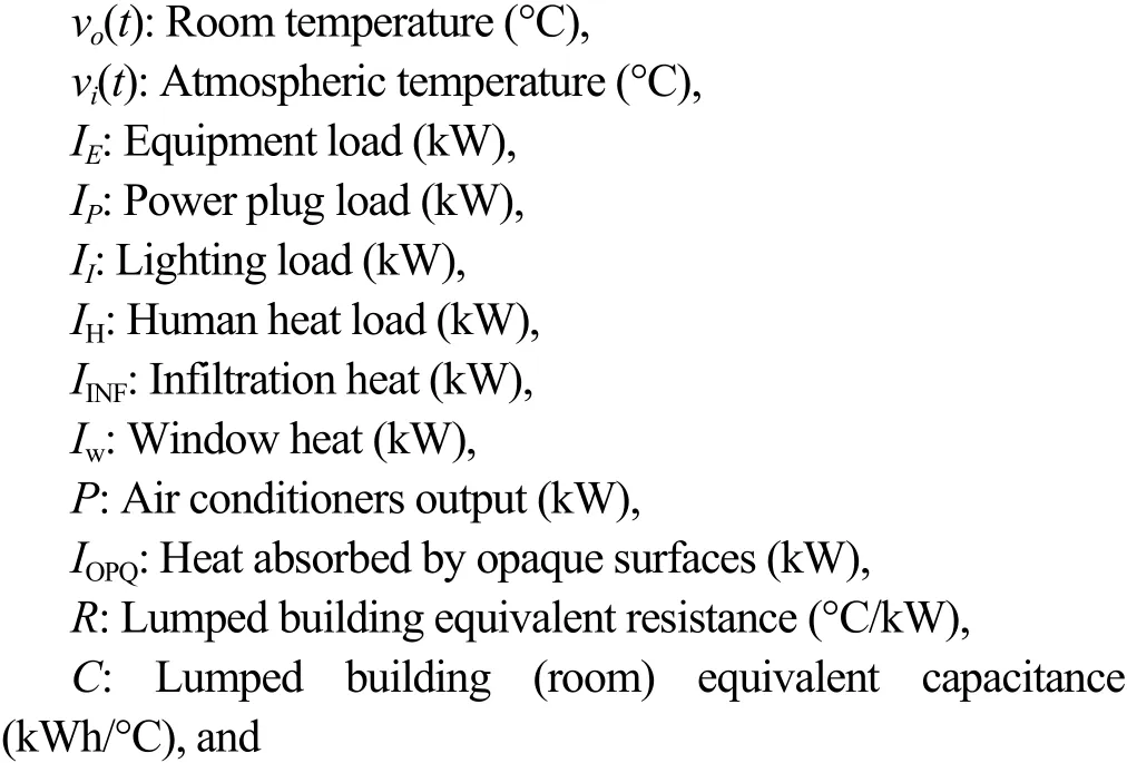
Fig. 11 is simplified by summing up all the loads as shown in Fig. 12 for deriving discrete equation:

For co-simulation of Simulink, BCVTB, and Energy Plus,the Simulink only allows the discrete mode. By using the Kirchhoff voltage law and electric thermal analogy, the discrete model of the RC network shown in Fig. 12 is derived[12],[20],[21]as follows:

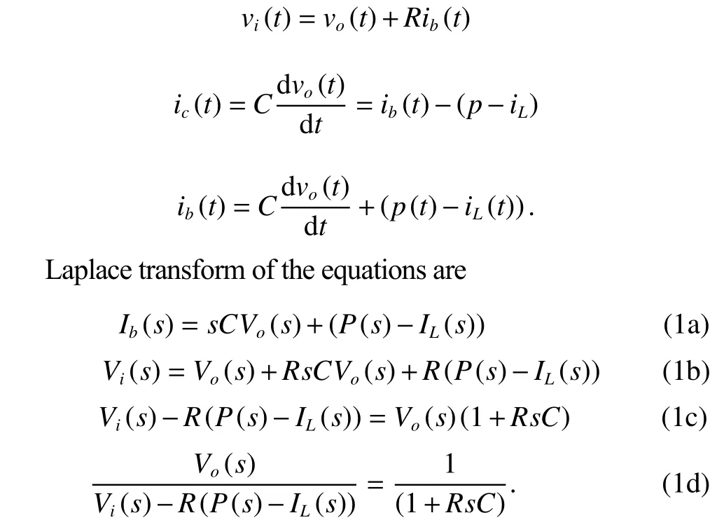
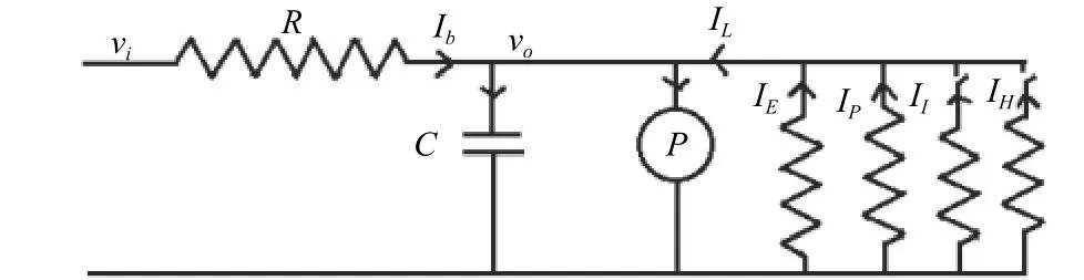
Fig. 11. Building Heat flow model.

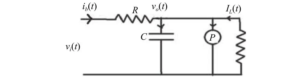
Fig. 12. Simplified building heat flow model.

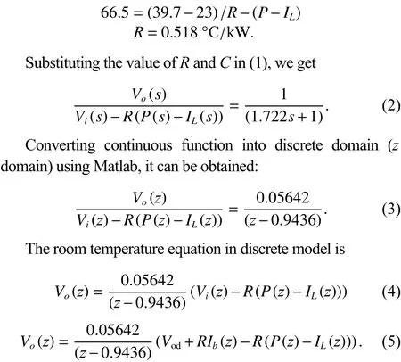
In the follows, we will calculate theRandCusing the building thermal parameters. The peak thermal load,comprising of building envelope heat, equipment heat load,power plug heat load, and human heat load works out to 66.5 kW. To find the lumped capacitanceC, by taking the temperature gradient

To find the lumped resistanceRof the building, with the air conditioner loadP=0 andIL=34.26 kW. The peak temperature during May for Chennai is taken as 39.7 °C and the room temperature is taken as 23 °C

3.2 Model Synchronization

Equation (4) represents the RC model which considers the variations ofVi(z) in °C. This is similar to the conventional model shown in [12], [13], and [19] to [22]. As per the method proposed in this paper, (5) considers the variation of the building fabric cooling load in kW obtained from Energy Plus.On the design day, the peak atmospheric temperature is

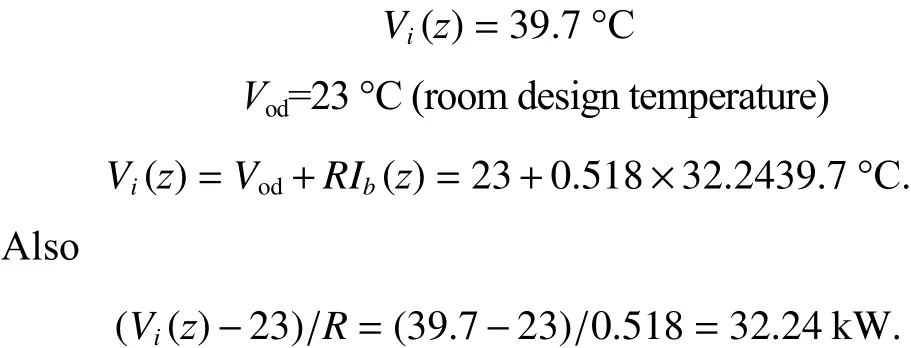
This 32.24 kW is the design day building fabric cooling load discussed in Section 3. The design day for this building falls on May 9. The RC model (4), EBACS model (5)proposed in this paper, and manual method of heat load calculations are synchronized for the design day.

4. Model Based Approaches for Improving Energy Efficiency

Simulations have been carried out for the comparison of scheduling scheme of air conditioners. Three methods are used for studying the air conditioner scheduling considering:

1) Equal state AC scheduling (ESACS)-current practice.

2) Day night AC scheduling (DNACS)-time based scheduling.

3) Energy balanced AC scheduling (EBACS)-computing the total thermal load.

Using the simulation model, the data ofIb(z) andVi(z) has been applied for Aug. 16.

The data used for simulation of various models is described below. The equipment loadIE(z) has been obtained from the site. The power plug load is kept constant and theII(z) andIH(z)are controlled by day night control. The Simulink diagram load block is shown in Fig. 13. The Ptolemy model indicated in Fig. 10 has been used for time synchronization and taking the output parameters.

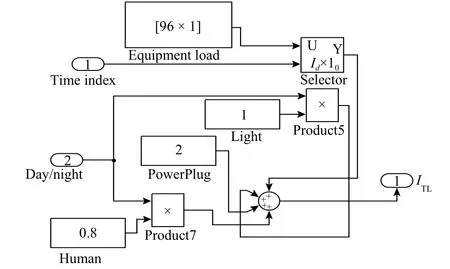
Fig. 13. Load block.

4.1 Equal State AC Scheduling (ESACS)

In this method, the climate influence on building fabric cooling load has been considered as atmospheric temperature variations. The atmospheric temperatureVi(z) and equipment loadIE(z) are stored as time series data and they are selected during simulation. TheIP(z) is fixed. TheII(z) andIH(z) are controlled by using day/night selection algorithm. The settings on thermostat arethe relay block acts as thermostat and controls the switch. The individual air conditioner feed cooling output is 7×3.5=24.5 kW. All the time, the full capacity is kept in operationN=3. So the total air conditioners capacity is 73.5 kW. Fig. 14 shows the part of ESACS scheduling scheme. Table 2 exhibits the legend for graphs.

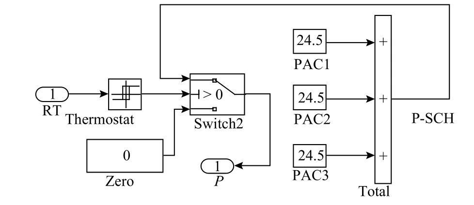
Fig. 14. ESACS scheduling scheme.

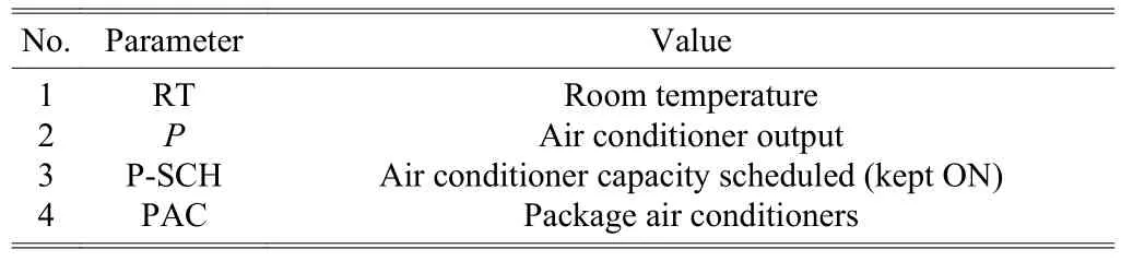
Table 2: Legend for graphs

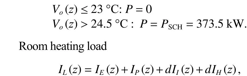
whered=1 during the day (10:00 to 18:00) andd=0 for the remaining time. The climate influence on building fabric cooling load has been considered as the variations ofVi(z)using (4). In this methodN=3 all the time. The simulation results of ESACS scheme for the day, Aug. 16, are shown in Fig. 15. This method does not apply the variations of thermal load in the scheduling of air conditioner. The control is based on room temperature-thermostat only. This results in the wastage of energy since full capacity of air conditioners has been put ON throughout the year

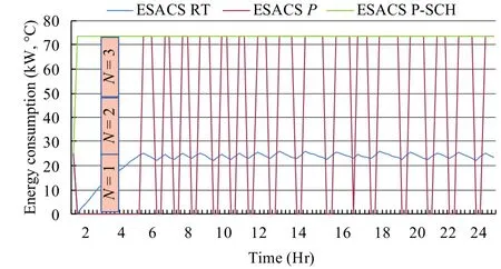
Fig. 15. ESACS scheduling on Aug. 16.

4.2 Day Night Air Conditioner Scheduling (DNACS)

In this scheme, 1/3 of the capacity of air conditioners is deliberately switched to OFF during the night hours. Fig. 16 shows part of the DNACS schedule. This is to reduce ofIb,IH,II, andIE. During the day time, the full capacity is switched ON.The advantage is that partial energy saved is over ESACS. This is based on the time factor only and the computation of fabric cooling load is not considered. The Simulink model is shown in Fig. 16. The climate influence on the fabric cooling load of building is considered as variations ofVi(z) using (4).

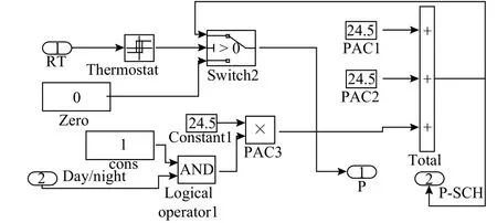
Fig. 16. DNACS scheduling.

The simulation with data on Aug. 16 has been plotted in Fig. 17 for DNACS scheme.

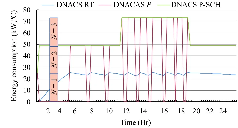
Fig. 17. DNACS scheduling on Aug. 16.

4.3 Energy Balanced Air Conditioner Scheduling(EBACS)

In this method, the air conditioner is scheduled proportional to the thermal load, by estimating the thermal load. TheIbcan be estimated in two ways:

1) In first way,Ib(z) which is the computed data of Energy Plus is used directly in time synchronized manner for every control step for one day. This method is called TIMTA. TheIb(z) has been obtained by using modeling and simulation as shown in Fig. 9 and Fig. 10 for the day of Aug. 16. It consists of 96 samples for each 15 minutes. Along withIb(z)atmospheric temperature is also obtained for the same duration.

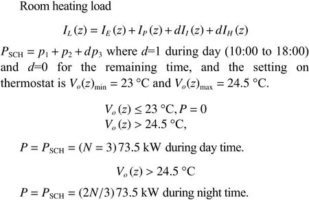
with fractional values rounded off to one, and wherepis the cooling capacity of individual air conditioners in kW,d=1 during the day time (10:00 to 18:00) andd=0 for the remaining time. The setting on thermostat is

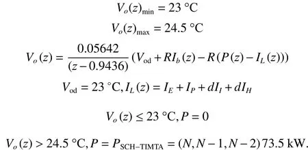
The capacity of the air conditioners is proportionally varied asN,N–1,N–2 by computing the thermal load. Fig. 18 shows the EBACS sheduling. Fig. 19 shows the results of EBACS scheduling with TIMTA.

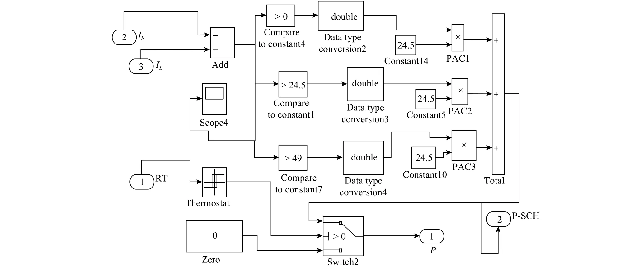
Fig. 18. EBACS scheduling.

Fig. 19. EBACS-TIMTA scheduling on Aug. 16.

PSCH-TIMTAis the air conditioner capacity put in to ON. This depends on various thermal loads including the fabric cooling load of the building envelopeIb(z) obtained from Energy Plus.

From Fig. 8, it can be seen that theIb(z) varies from the maximum during May to zero during most of the time in January.PSCH-TIMTAaccounts for the variations of thermal load includingIb(z). This avoids over cooling and increases the energy efficiency.

2) The other method called TEMTIM, in whichIbhas been curve fitted over the atmospheric temperatureVi(z) obtained for the same period. This facilitates simplified computation ofIbby usingVi(z). This method of computingIbis called the virtual sensing method. This method applies the measured atmospheric temperature.

The constantsa,b, andcobtained by curve fitting have been indicated in Table 3.

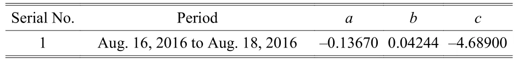
Table 3: Linear curve fitting constant values

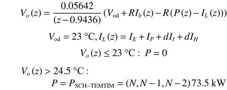
whered=1 during the daytime (10:00 to 18:00) andd=0 for remaining time. The setting on thermostat

PSCH-TEMTIMalso estimates the total load for scheduling of the air conditioners. Fig. 20 shows the block diagram of virtual sensing method. Fig. 21 shows the results of the EBACSTEM TIM scheduling.

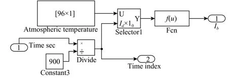
Fig. 20. Virtual sensing method.

The EBACS scheduling shown in Fig. 18 has been used in this scheme also. ButIb(z) has been computed using (6).

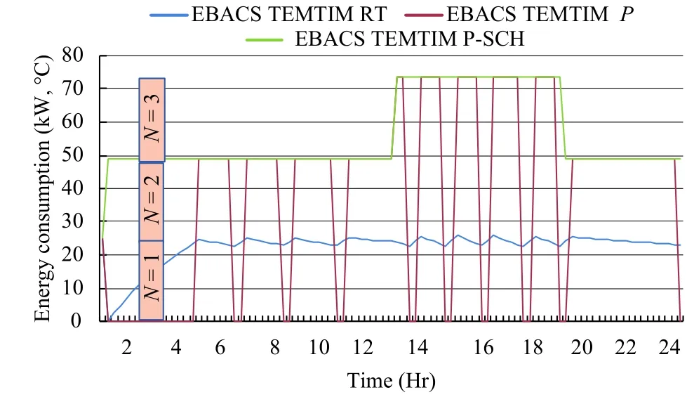
Fig. 21. EBACS-TEMTIM scheduling on Aug. 16.

5. Field Experiment

5.1 Hardware Setup

Field experiment has been conducted in building under study. Three numbers 7 TR PACs are feeding the equipment room with one 7 TR PAC as standby. The designated master PAC controls the sequence of operation. During the test period,the sequencing was discontinued and three air conditioners are used for testing. In the equipment room, the air flow to the racks was adjusted by adjusting the fixed volume control dampers. The temperature distribution in the room was uniform. The PAC works by sensing the temperature of the return air. The minimum set point was 23 °C and maximum set point was 24.5 °C in the return air. The allowed room temperature range is 23 °C to 26 °C. The RH range is 30% to 60% due to climate, and the comfortable RH is maintained inside, without activation of the heater. The cooling capacity of the air conditioners was calculated by measuring the cubic foot per minute (CFM) of air quantity, inlet and outlet temperatures.For simplicity of the calculation, the capacity was calculated in tonnage kW using (7) as shown in Table 4.

Figs. 22 and 23 show the hardware set up used for field study and Fig. 24 shows the view of PACs. Fig. 25 shows the software used for recording of the field parameters.

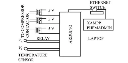
Fig. 22. Hardware configuration for measurement.

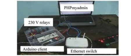
Fig. 23. Hardware setup for measurement.

Fig. 24. Group of PACs.

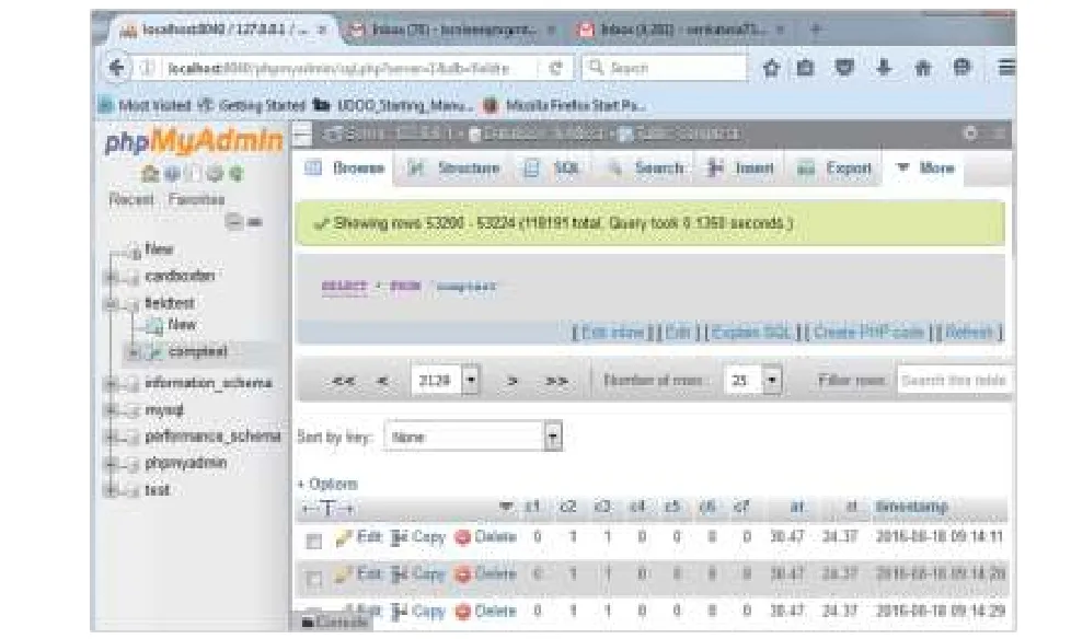
Fig. 25. XAMPP PHP myadmin database server page.

The room temperature, atmospheric temperature, and the ON/OFF time of the compressor are recorded using embedded Ethernet setup designed for this purpose as shown in Fig. 23. It comprises of the Arduino microcontroller, relays, and temperature sensors. The software XAMPP (X-operating system, A-Apache server web server, M-My SQL, PHP-language, and PERL language) installed in the laptop can receive the data collected by the Arduino micro controller with Ethernet board. From the XAMPP database the recorded data has been converted as Excel data for the analysis purpose.

The period of simulations was the same as that of field study. The following sections discuss the results of field study.

5.2 Record of DNACS Scheduling during Aug. 13, 2016 to Aug. 14, 2016

The record of DNACS scheduling during Aug. 13, 2016 to Aug. 14, 2016 is shown in Fig. 26, where FT is the field test,CP is the current practice, RT means the room temperature(°C), P-SCH is the air conditioner capacity scheduled (kW),Pis the cooling output of air conditioners (kW), and ITL is the total thermal load (kW). The DNACS scheduling scheme simply relies on time factor only. During the daytime from 10:00 to 18:00 three (N=3) PACs were put ON and remaining time only two air conditioners were kept ON. The compressor on time and the room temperature are plotted in Fig. 26 (e).

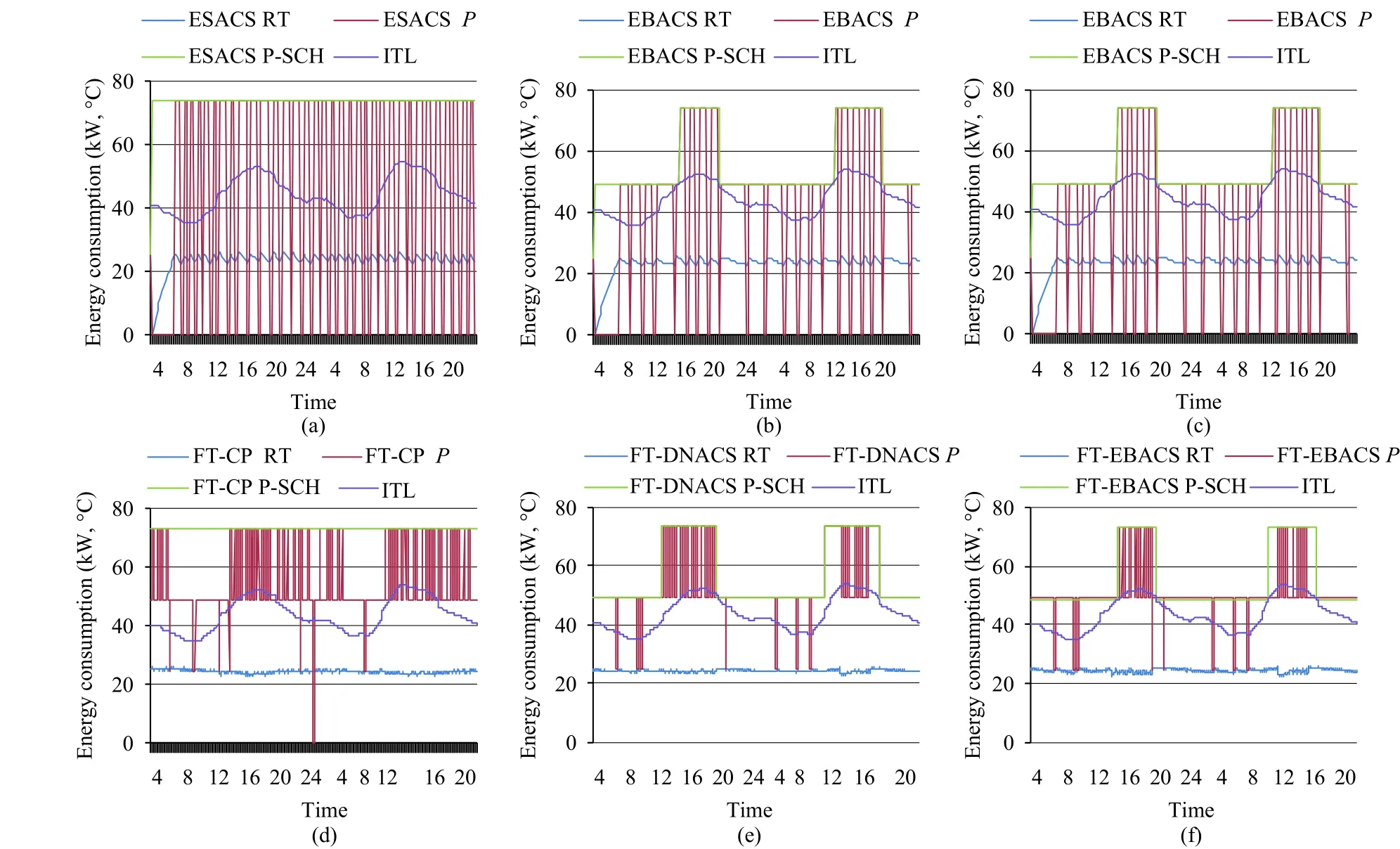
Fig. 26. Results of simulations and field experiment: (a) ESACS simulations during Aug. 15, 2016 to Aug. 16, 2016, (b) DNACS simulations during Aug. 13, 2016 to Aug. 14, 2016, (c) EBACS simulations during Aug. 17, 2016 to Aug. 18, 2016, (d) ESACS field test during Aug. 15, 2016 to Aug. 16, 2016, (e) DNACS field test during Aug. 13, 2016 to Aug. 14, 2016, and (f) EBACS field test during Aug. 17, 2016 to Aug. 18, 2016. The EBACS scheduling brings lesser duration of air conditioner.

5.3 Record of Current Practice ESACS during Aug. 15,2016 to Aug. 16, 2016

The current practice of working of the air conditioners recorded for the day Aug. 15, 2016 to Aug. 16, 2016. The record of scheduling capacity, actual compressor ON/OFF, and room temperature has been shown in Fig. 26 (d). In current practice, all (N=3) air conditioners kept ON throughout the day Aug. 16. The compressors turn ON whenever the room temperature goes above the set point, without adapting to the thermal load.

5.4 Scheduling with EBACS during Aug. 17, 2016 to Aug. 18, 2016

Fig. 26 (f) shows the recorded data based on EBACS scheduling during Aug. 17, 2016 to Aug. 18, 2016. As shown,the duration of the third compressor ON is restricted by scheduling based on the computed total thermal load. The thermal load is less in the night time and in the morning, i.e.less than 49 kW, so 2 PACs are sufficient (N–1). The thermal load exceeds 49 kW in the midday i.e. during 13:00 to 18:00. So 3 (N) air conditioners are put ON during these period. This duration may change during summer and winter.Interestingly, the EBACS scheduling brings energy efficiency and avoids more capacity of air conditioners kept ON than the required capacity for every control step. As shown in Fig. 26(f) the room temperature did not exceed the specified range of(23±3) °C.

6. Results and Discussion

The energy consumed by different scheduling schemes during simulations and field experiment study discussed above has been indicated in Table 5. The method ESACS is equivalent to the current practice, consumes more energy than the other schemes. The DNACS scheme consumes slightly less than the ESACS scheme and it is not an accurate method. In contrast, the EBACS scheme consumes less than the ESACS and DNACS. Thus, the EBACS scheme has the potential of energy savings. Also, during the full year simulation study, the energy consumed by the various schemes is indicated in Fig.27. As shown in Fig. 27 the EBACS consumes less energy than the other schemes, and about 4% energy savings has been obtained over ESACS scheme.

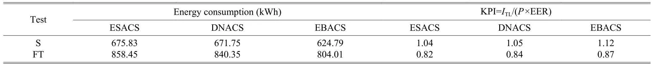
Table 5: Comparison energy consumption and KPI index of various scheduling scheme for the period Aug. 13, 2016 to Aug. 18, 2016

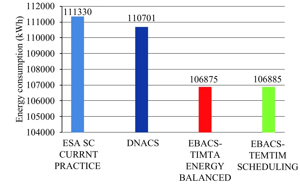
Fig. 27. Comparison of energy consumption during simulation for the whole year.

According to [24], the healthiness of the air conditioners is good only when the key performance index (KPI) is between 0.9 to 1.1. In this work, the KPI for different scheme is shown in Table 6. In case of ESACS and DNACS, the KPI value is an indicative representation only. Since the practically thermal load did not compute in these schemes, as the out of three schemes mentioned, the EBACS gives a higher KPI index compared with other schemes. In the EBACS scheme, the fault in the air conditioner can be immediately detected. The ESACS and DNACS methods are independent of the thermal load, so fault detection is difficult.

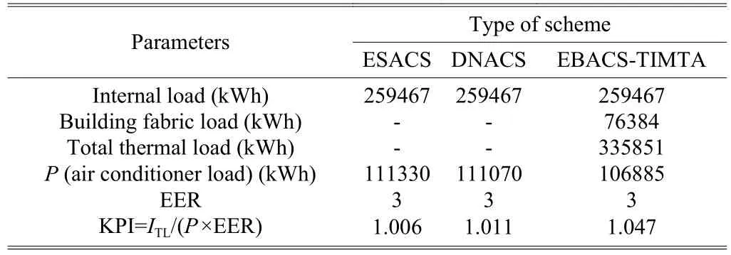
Table 6: KPI index of various scheduling scheme for whole year

7. Conclusions

The air conditioner scheduling problem for round the clock operated building has been addressed in this paper. The thermal load computation problem has been addressed by software based pre-computation. Three strategies have been analyzed and compared. The EBACS method which uses the computed fabric cooling load saves more energy than the other two methods. Thus computing the thermal load is the most efficient approach for scheduling and fault detection. By modeling and simulation the optimal cooling opacity can be arrived for scheduling of air conditioners with optimization energy consumption.

The EBACS-TIMTA and EBACS-TEMTIM method facilitate the air conditioner capacity reduction automatically.The existing practice does not consider the thermal load for every control step. But the total thermal load goes even below 50% during winter season. Energy Plus can be used for modeling any building and simulation can be made using the climate data. Using the interfacing method described in this paper, the fabric cooling load of the building envelope can be acquired for the control and scheduling purposes to improve energy efficiency. This software aided model based precomputation can help climate adaptive cooling capacity control instead of continuing the peak capacity all the time. It also helps for fault detection using the KPI based index. Thus, the proposed EBACS method has the potential of energy saving in round the clock operated buildings and other buildings for energy conservation and fault detection.

Acknowledgment

The authors express their acknowledgement for the support and facilities provieded by Bharat Sanchar Nigam Limited Chennai Telephones and Department of Telecommunications,India for this study.