POSITIVE SOLUTIONS FOR A WEIGHTED FRACTIONAL SYSTEM∗
2018-07-23PengyanWANGYongzhongWANG
Pengyan WANG()Yongzhong WANG()
Department of Applied Mathematics,Northwestern Polytechnical University,Xi’an 710129,China
E-mail:wangpy119@126.com;wangyz@nwpu.edu.cn
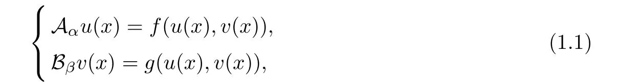
Abstract In this article,we study positive solutions to the system
Key words Weighted fractional system;positive solution;radial symmetry;monotonicity;non-existence
1 Introduction
This article concerns to the weighted fractional system
where
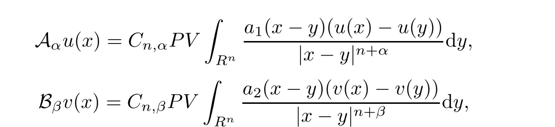
(I)aiis radial decreasing,this is,for any x,y∈Rn,we havewith|x|≤|y|;there exists two positive constants m and M such that m≤ai(x−y)≤M.
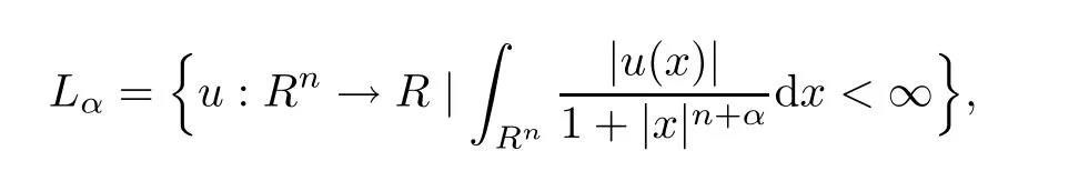
and Lβis defined similarly.
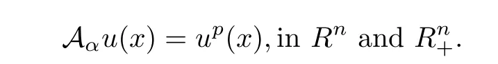
The operator Aαis weighted fractional Laplacian and arises from purely jump Lévy processes.It also appears in stochastic control problems[10].Caffarelli and Silvestre have proved the regularities to nonlocal equations in[2,3].If a1(x)≡1,then

The nonlocal nature of fractional operators brings many new difficulties comparing with the usual Laplacian.To treat fractional operators,Caffarelli and Silvestre[4]raised the extension method which turns the nonlocal problem involving the fractional Laplacian into a local one in higher dimensions.Another method to deal with the nonlocal difficulty is to consider the equivalent integral equation corresponding to the fractional Laplacian equation.Recently,equations involving the fractional Laplacian have been extensively studied,which were used to model diverse physical phenomenas,such as quasi-geostrophic flow,anomalous diffusion,posudo-relativistic boson stars,and boundary control problems;see[1,5,9]and the references therein.Till now,the few deals with equations involving different orders and weighted fractional Laplacian.
Chen,Li,and Li[7]developed a new method that can be used to directly on the nonlocal operator.For example,the direct method of moving planes in[7]had been extended to fully nonlinear nonlocal operator Fα(see[6]).For more articles concerning the method of moving planes for nonlocal equations and integral equations;see[8,12,13,17]and the references therein.Tang[15]studied the weighted fractional equation,

and
For the weighted fractional Laplacian,so far as we know,there is neither any corresponding extension method nor equivalent integral equations that one can work at.The motivation of this article is to generalize the direct method of moving planes to the problems involving weighted fractional operators

and
Compared with the single equation in[15],the research to systems meets some new difficulties.One of difficulties is that the coupling between solutions to(1.1)needs to be considered.To overcome these difficulties,we have to utilize a new idea–the iteration method–to establish a narrow region principle and a decay at infinity,which is inspired by a previous work by Li and Ma[11]and is a key point of this article.
Let us state the main results of this article.
Theorem 1.1Assume thatandare positive solutions to system(1.2)with f(·)and g(·)being Lipschitz continuous in the range of u(x)and v(x).Ifthen u(x)and v(x)are radially symmetric and monotone decreasing about the origin.
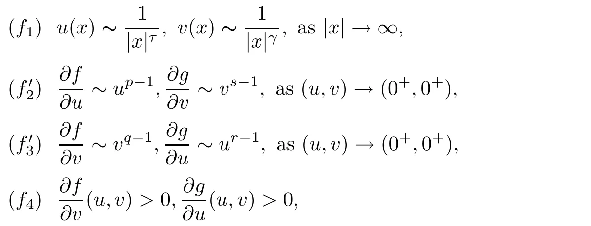
Theorem 1.2Assume thatandare positive solutions to system(1.3)with f,g∈C1([0,+∞)×[0,+∞),R).Suppose that

(f5) α
A consequence of Theorem 1.2 is the radial symmetry for the system

Corollary 1.3Letandbe positive solutions to(1.5)with the following conditions:
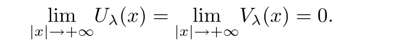
(f1)as|x|→ ∞;

Then,u(x)and v(x)are radially symmetric and monotone decreasing about some point x0in
Theorem 1.4Assume thatandare positive solutions to system(1.3)with f,g∈C1([0,+∞)×[0,+∞),R).Suppose that
Then,u(x)and v(x)are radially symmetric and monotone decreasing about some point x0in Rn.
Remark 1Theorem 1.2 is a generalization of Theorem 3 in[15]and Theorem 1 in[14].Theorem 1.4 generalizes Theorem 3 in[15]and Theorem 4 in[14].When ai(x−y)=1,α=β,Theorems 1.2 and 1.4 are reduced to a fractional Laplacian version of Theorem 1 and Theorem 4 in[14],respectively.
As an application,we apply Theorem 1.4 to the following system
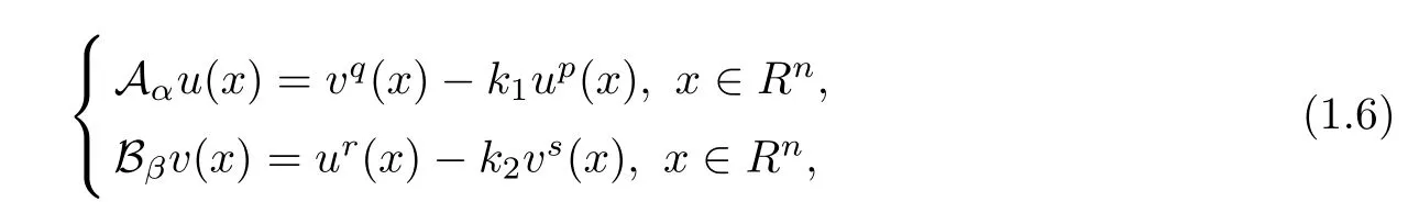
and obtain the radial symmetry property for the decay solution.
Corollary 1.5Letandbe positive solutions to(1.6)with the conditions:
(f1)
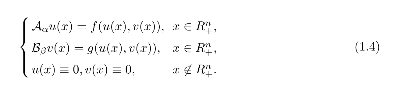
Theorem 1.6Assume thatare nonnegative solutions of system(1.4).Suppose that f and g are nonnegative.u(x)and v(x)are lower semicontinuous onand satisfy eitherThen,
Thie article is organized as follows.In Section 2,we establish the narrow region principle and decay at infinity.Section 3 is devoted to the proofs of Theorems 1.1,1.2,1.4 and Corollaries 1.3,1.5 by using the previous results and the method of moving planes.In Section 4,we prove Theorem 1.6.
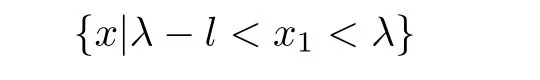
For simplicity,we list some notations used frequently:for λ ∈ R,denoteλ}and xλ=(2λ − x1,x2,···,xn).Set

Throughout this article,C will be the positive constant depending on m,M,n,α,which can be different from line to line.
2 Narrow Region Principle and Decay at In finity
Ley us use the iteration method to establish the narrow region principle and decay at infinity,which play important roles in applying the direct method of moving planes.Denote
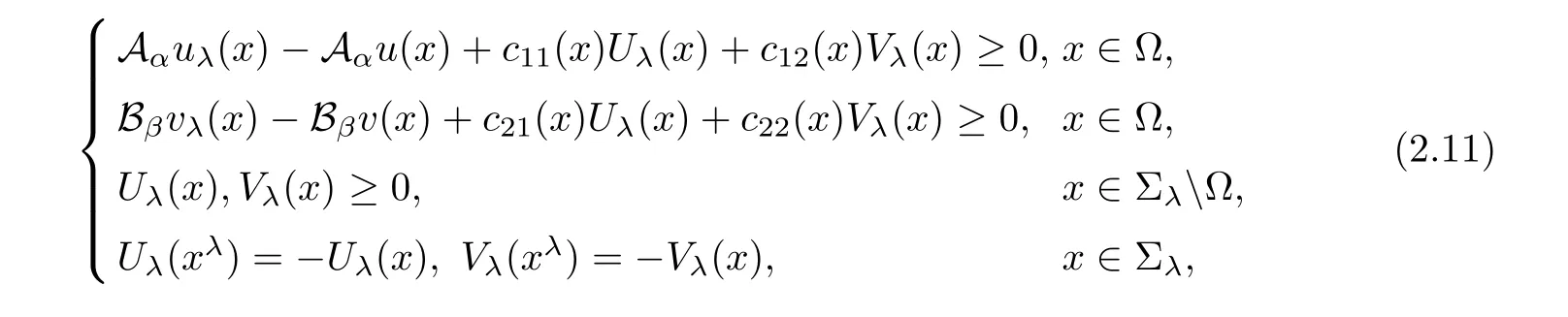
Theorem 2.1(Narrow Region Principle) Let Ω be a narrow region in Σλand lie in
with small l>0.Suppose thatandare lower semi-continuous on,and satisfy
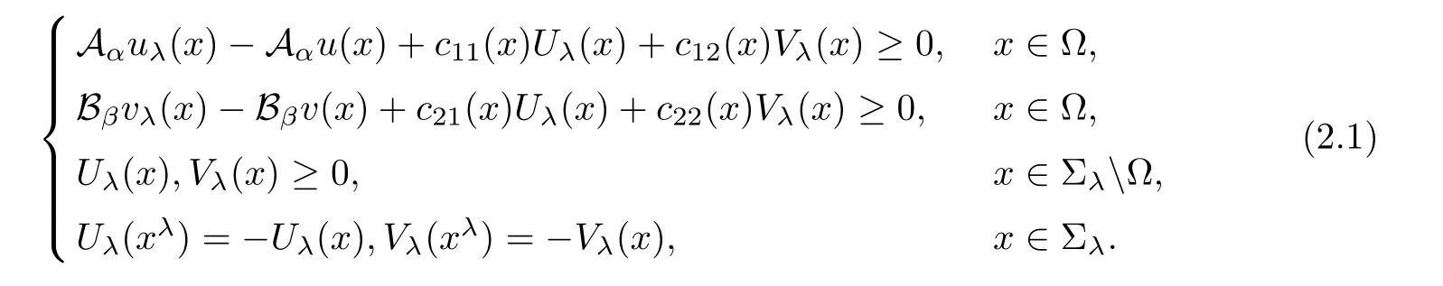
(i)If cij(x)(i,j=1,2)are bounded from below on a bounded domain Ω,c12(x)<0,and c21(x)<0 on Ω,then we have,for sufficiently small l,

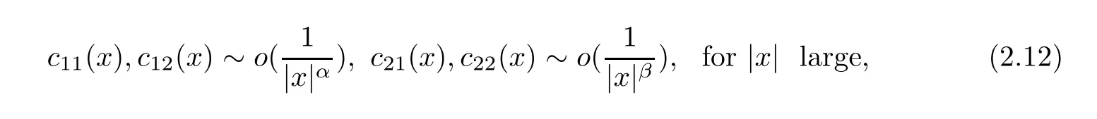
(ii)If Ω is unbounded,then conclusion(2.2)still holds under the additional conditions

(iii)Furthermore,under the conditions of(i),if either Uλ(x)or Vλ(x)attains 0 somewhere inΩ,then

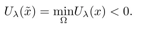
Proof(i) If(2.2)does not hold,without loss of generality,we assume that Uλ(x)is negative at some point in Ω.Then,the lower semi-continuity of Uλ(x)onguarantees that there exists some∈Ω such that


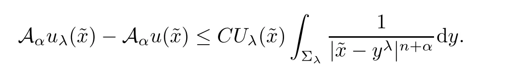
Similar to[11],we have
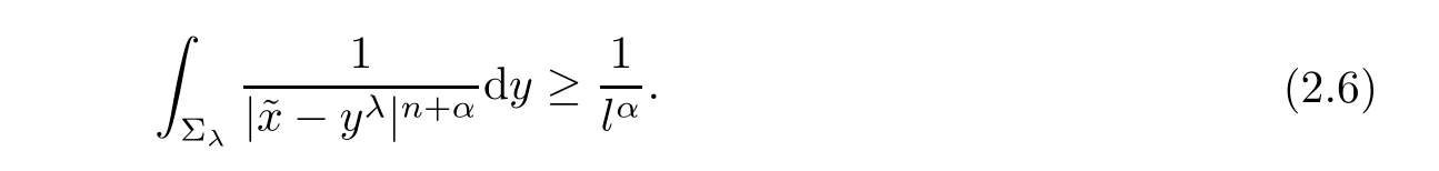
Putting(2.6)into(2.5),
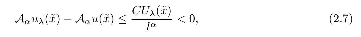
and noting the assumption on c11(x),

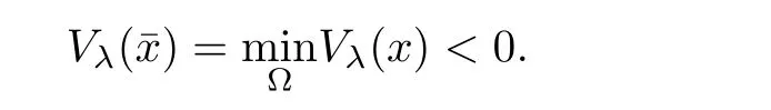
It follows from(2.1)and(2.8)that

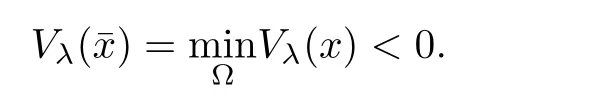
With(2.9)and the lower semi-continuity of Vλ(x)on Ω,we know that there existssuch that
A similar argument to(2.8)derives that

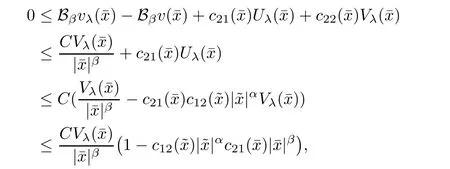
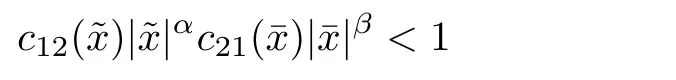
Combining it with(2.1),(2.9),and the assumptions on c12(x)and c21(x),we have,for l sufficiently small,
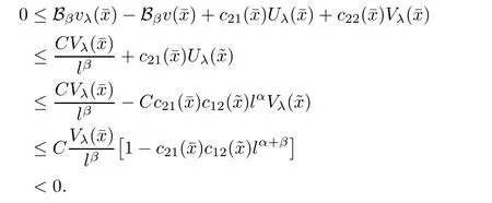
This contradiction shows that(2.2)must be true.
(ii)If Ω is unbounded,then(2.2)is easily obtained using(2.3).
(iii)Next,we prove(2.4).Without loss of generality,suppose that there exists η ∈ Ω such that

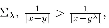
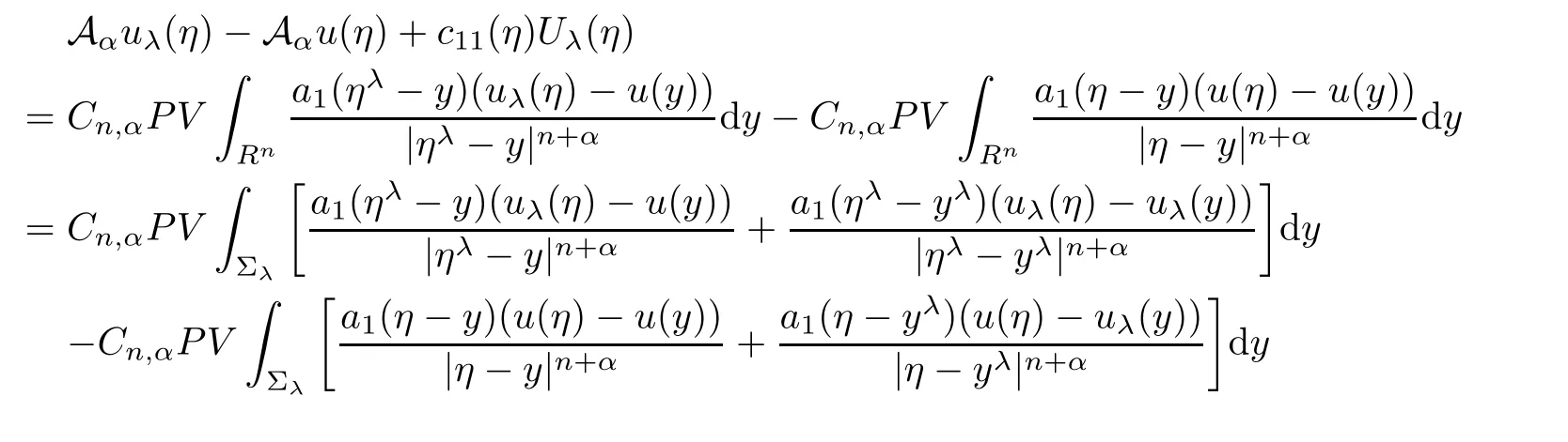

Using it and(2.1),we see that Vλ(η)<0.This contradicts(2.2).Hence,in Σλ.From the first equation in(2.1),it gives

Because we already know
we have

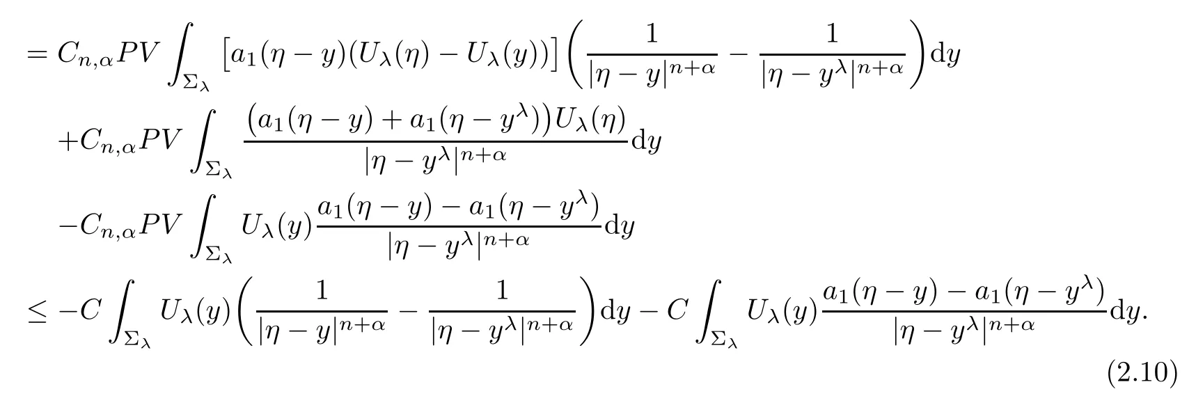
Similar to(2.10),we get

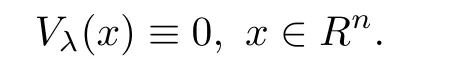
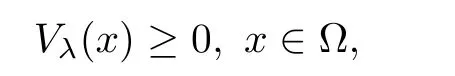
Similarly,one can show that if Vλ(x)attains 0 at one point in Σλ,then both Uλ(x)and Vλ(x)are identically 0 in Rn.Thus,this completes the proof. ?
Remark 2We call(iii)the strong maximum principle later.As we can see from the proof,to conclude(2.4),Ω can be unbounded and Ω does not need to be narrow.
Theorem 2.2(Decay at In finity) Let Ω be an unbounded domain in Σλ.Assume thatare lower semi-continuous onand Uλ(x)and Vλ(x)satisfy
with
and

If Uλattains a negative minimum atand Vλattains a negative minimum atin Σλ,then there exists a positive constant R0depending only on cij(x)such that

ProofBy the assumptions,there exists∈Ω,such that
By inequality(2.5),
For each fixed λ∈R,there exists a positive constant c such that if||is large enough,then(see[16]),
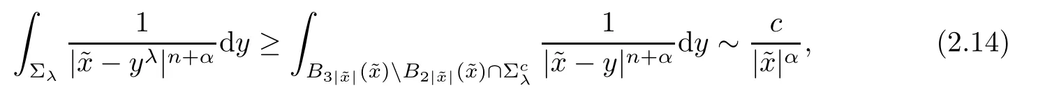
hence

From(2.15)and(2.11),it is easy to deduce that

and

Similar to(2.15),we derive

Combining(2.11),(2.12),(2.16)and(2.18),it follows that for λ sufficiently negative,
Remark 3(I)As the x1direction can be chosen arbitrarily,Σλchanges following the change of x1direction,so the results of Theorems 2.1 and 2.2 for the other direction hold.
(II)If Uλ(x)has a negative minimum atin Σλ,then Vλ(x)attains its negative minimum atand vise versa.
3 Symmetry of Solutions in B1(0)and Rn
On the basis of Theorems 2.1 and 2.2,we apply a direct method of moving planes to obtain symmetry and monotonicity of positive solutions to(1.2)in B1(0)and(1.3)in Rn.
Proof of Theorem 1.1Choose an arbitrary direction as the x1-axis.LetB1(0)|x1=λ},
Step 1We prove that for λ>−1 sufficiently close to−1,

It is easy to verify that
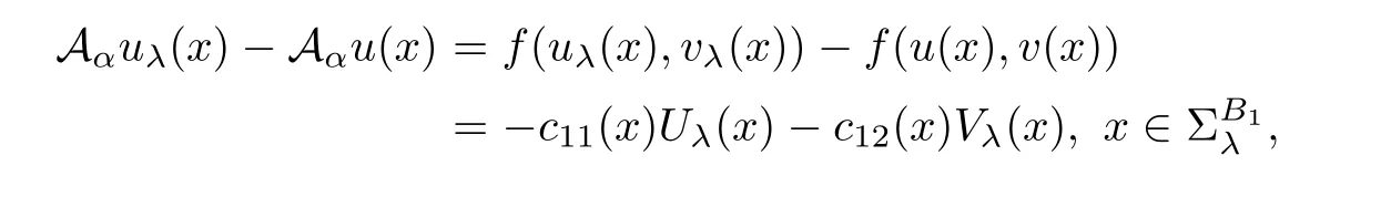
and
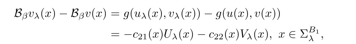
where

and

The Lipschitz continuity assumption on f and g guarantees that cij(x)are uniformly bounded from below and the fact thatandmeans that c12(x)<0 and c21(x)<0.Therefore,Theorem 2.1 gives that(3.1)holds for λ > −1 sufficiently close to-1.
Step 2Keep moving the planes to the limiting positionas long as(3.1)holds.
Setting

we claim

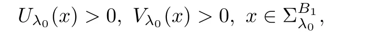
Indeed,by the contraction,we suppose λ0<0.As Uλ0(x)≥ 0 and Vλ0(x)≥ 0 butand,from(iii)in Theorem 2.1,we have
and then there exist a positive constants c0such that for any δ>0,

From the continuity of Uλ(x)and Vλ(x)with respect to λ,we see that there exists a positive constant ǫ,such that for all λ ∈ (λ0,λ0+ ǫ),

Via Theorem 2.1,it implies that

and so

which contradicts the definition of λ0.Therefore,λ0=0.
It follows that

that is,

As the x1direction can be chosen arbitrarily,(3.3)leads to that u(x)and v(x)are radially symmetric about the origin.The monotonicity is a consequence of the fact that Uλ(x)≥ 0 and Vλ(x)≥ 0 for anyand−1<λ≤0.
Next,let us prove Theorem 1.2.
Proof of Theorem 1.2Choose an arbitrary direction as the x1-axis.Denote Σλ={x∈Rn|x1<λ}.
Step 1Start moving the plane Tλfrom −∞ to the right in the x1-direction.
We will show that for λ sufficiently negative and any x ∈ Σλ,

By contradiction,without loss of generality,suppose that Uλ(x)is negative at some point in Σλ.By(f1),we have
Clearly,Uλ(x)=0 for x ∈ Tλ,and we know that Uλ(x)is negative in Σλ.Then,Uλ(x)must allow a negative minimum atin Σλ.Following the proof of Theorem 2.2,we find Vλ(x)attains a negative minimum atin Σλ.
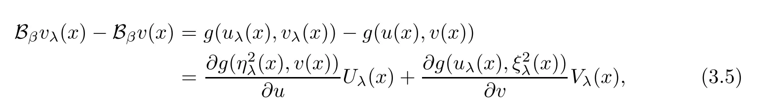
By the mean value theorem and(1.3),it yields that
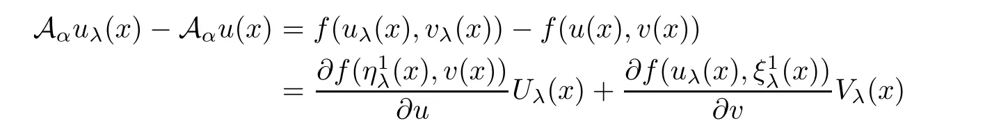
and
Consequently,it follows from Theorem 2.2 that

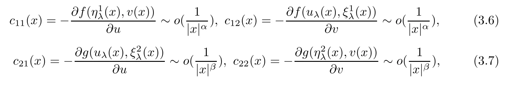
that is,for λ sufficiently negative(or|λ| It follows that Vλ(x)≥0 in Σλ.Otherwise,there existsin Σλsuch that and then from(2.18),we have Furthermore, However,combining(3.5)and(f4),we have The contradiction shows that Vλ(x)cannot attain its negative value in Σλ. This contradicts to the hypothesis and derives that(3.4)must be true.It completes the preparation for the moving planes. Step 2Keep moving the planes to the limiting position Tλ0as long as(3.4)holds. Letting we conclude Otherwise,if λ0= ∞,then for any λ >0,we obtain This is a contradiction and(3.11)is proved. Now,we point out that Otherwise,one can verify that there exists ǫ>0,such that for any λ ∈ (λ0,λ0+ ǫ), This will contradict to the definition of λ0and(3.12)is true. The remaining task is to prove(3.13)using Theorem 2.1 and Theorem 2.2. If Uλ0(x) ≥ 0 andbutand,from(iii)in Theorem 2.1,we have Let R0be the constant in Theorem 2.2.It follows that for any δ>0, Using the continuity of Uλ(x)and Vλ(x)with respect to λ,there exists a positive constant ǫ,such that for all Suppose that(3.13)is false,then either Uλ(x)is negative or Vλ(x)is negative at some point in Σλ.From the proofs of Theorem 2.1 and Theorem 2.2,we know that there existandsuch thatLet us consider three possibilities. Case 1 From(2.9),we have and Hence, Case 2Tand Proof of(3.13)is similar to Case 1.Here,we omit the proof. Case 3 By(2.7), where l= δ+ǫ.Combining it and(2.1),it implies Similar to(3.17),we derive Noting(3.18),then for l sufficiently small,it gives This contradiction shows that(3.13)has to be true. Now,we have proved that Uλ0(x)≡ 0,Vλ0(x)≡ 0,x ∈ Σλ0.As the x1direction can be chosen arbitrarily,we actually indicate that u(x)and v(x)are radially symmetric about some point x0.Also,the monotonicity follows easily from the argument.This completes the proof of Theorem 1.2. ? Proof of Corollary 1.3Setand g(u(x),v(x))=Picking 0 we can easily check that all the assumptions in Theorem 1.2 are satisfied. ? Proof of Theorem 1.4The proof is quite similar to the one of Theorem 1.2.Examining carefully the proof of Theorem 2.2,we see that if the assumptions(f2),(f3),and(f5)are replaced byandrespectively,the calculation process of(3.6),that is, is replaced by The rest of the calculations is similar.We still have the fact that(3.6)and(3.7)were established.So do the conclusions of Theorem 2.1 and Theorem 2.2.Therefore,it is straightforward to show Theorem 1.4.The details of the proof will be omitted. ? Proof of Corollary 1.5Let f(u(x),v(x))=vp(x)−k1ur(x),g(u(x),v(x))=uq(x)−k2vs(x).Choosing α We investigate problem(1.4). Proof of Theorem 1.6Noting(f1),it is easy to know that but Aαu(x)=f(u(x),v(x))≥ 0,which is impossible.If u(x)or v(x)attains 0 somewhere inthen In what follows,we always assume that u(x)>0 and v(x)>0 in.Let us carry on the method of moving planes on the solution u along the xndirection. Step 1For λ sufficiently small,it follows immediately that Step 2As(4.1)provides a starting point,we can move the planeupward as long as(4.1)holds.Defining we point out that Otherwise,if λ0< ∞,then the planecan be moved further upward.To be more rigorous,we can claim that there exists ǫ>0,such that for any λ ∈ (λ0,λ0+ ǫ), This will be a contradiction with the definition of λ0and hence(4.2)holds. Now,we prove(4.3).Using Theorem 2.1,Theorem 2.2,and the similar arguments in the proof of Theorem 1.2,it follows that which implies This is impossible,because we have assumed that u(x)and v(x)>0 in At this stage,(4.2)is valid and u(x)and v(x)are increasing with respect to xn.This contradicts to(f1)and the proof of Theorem 1.6 is ended. ?


4 Non-Existence of Solutions on a Half Space


杂志排行
Acta Mathematica Scientia(English Series)的其它文章
- GLOBAL EXISTENCE OF CLASSICAL SOLUTIONS TO THE HYPERBOLIC GEOMETRY FLOW WITH TIME-DEPENDENT DISSIPATION∗
- NONNEGATIVITY OF SOLUTIONS OF NONLINEAR FRACTIONAL DIFFERENTIAL-ALGEBRAIC EQUATIONS∗
- GROWTH AND DISTORTION THEOREMS FOR ALMOST STARLIKE MAPPINGS OFCOMPLEX ORDER λ∗
- EXACT SOLUTIONS FOR THE CAUCHY PROBLEM TO THE 3D SPHERICALLY SYMMETRIC INCOMPRESSIBLE NAVIER-STOKES EQUATIONS∗
- PRODUCTS OF RESOLVENTS AND MULTIVALUED HYBRID MAPPINGS IN CAT(0)SPACES∗
- CONVERGENCE FROM AN ELECTROMAGNETIC FLUID SYSTEM TO THE FULL COMPRESSIBLE MHD EQUATIONS∗