Seasonal variation and modal content ofinternal tides in the northern South China Sea*

GUO Zheng (郭筝) CAO Anzhou (曹安州) LÜ Xianqing (吕咸青)

1Physical Oceanography Laboratory/CIMST,Ocean University of China,Qingdao 266100,China

2Qingdao National Laboratory for Marine Science and Technology,Qingdao 266100,China

3Ocean College,Zhejiang University,Zhoushan 316021,China

AbstractA nine-month mooring record was used to investigate seasonal variation and modal content ofinternal tides (ITs) on the continental slope in the northern South China Sea (SCS). Diurnal tides at this site show clear seasonal change with higher energy in winter than in spring and autumn, whereas semidiurnal tides show the opposite seasonal pattern. The consistency ofiTs with barotropic tides within the Luzon Strait, which is the generation region of the ITs, implies that the seasonal variation ofiTs depends on their astronomical forcing, even after extended propagation across the SCS basin. Diurnal tides also differ from semidiurnal tides in relation to modal content; they display signals of high modes while semidiurnal tides are dominated by low modes. reflection of the diurnal tides on the continental slope serves as a reasonable explanation for their high modes. Both diurnal and semidiurnal tides are composed of a larger proportion of coherent components that have a regular 14-day spring-neap cycle. The coherent components are dominated by low modes and they show obvious seasonal variation, while the incoherent components are composed mainly of higher modes and they display intermittent characteristics.

Keyword:internal tide (IT); South China Sea (SCS); seasonal variation; modal content

1　INTRODUCTION

The South China Sea (SCS) has long been identified as a site ofintense internal tide (IT) activity due to its characteristic double meridional submarine ridges,strong stratifi cation, and astronomical tides. These strong ITs are considered a primary cause of the enhanced diapycnal mixing and the occurrence of strong nonlinear internal solitary waves in the SCS(Tian et al., 2009; Huang et al., 2016, 2017), which are important for driving or modulating the SCS deep circulation (Zhao et al., 2014; Zhou et al., 2014; Dong et al., 2015). Therefore, ITs in the SCS have been studied in different ways over past decades. For example, Jan et al. (2008) used a three-dimensional tide model to investigate the spatiotemporal variations of baroclinic tides in the Luzon Strait (LS). Vlasenko et al. (2010) focused on the vertical structure ofiTs in the SCS in their modeling efforts. In addition to numerical model simulations, in situ data have also been analyzed to further the understanding of the internal wave fi eld of the SCS. Extensive current moorings were deployed around the continental shelfbreak area in the northern SCS during the Asian Seas International Acoustic Experiment, enabling the study ofiTs and nonlinear internal wave behavior (Duda et al., 2004; Liu et al., 2004; Duda and Rainville, 2008).Using the fi rst comprehensive set of observations obtained during the Internal Waves in Straits Experiment, in combination with high-resolution numerical modeling, Alford et al. (2015) described the complete evolution ofinternal waves in the SCS.They showed that the waves begin as ITs, steepen dramatically as they propagate west from the LS, and then shoal onto the continental slope to the west.Based on satellite altimetric measurements, which provide an important solution to the lack of fi eld observations, Zhao (2014) provided a picture of the propagation and distribution of the K1, O1, and M2ITs from the LS.

In addition to ITs, the northern SCS has abundant strong mesoscale eddies that arise from the Kuroshio intrusion (Zhang et al., 2013, 2017). Because the Kuroshio intrusion and associated eddy shedding occur primarily in winter (Zhang et al., 2015, 2017),they strongly modulate the seasonal variation of the horizontal and vertical density distribution (or stratifi cation) in the northern SCS. Unsurprisingly,the seasonal density variation in combination with other season-dependent factors (Shaw et al., 2009;Buijsman et al., 2010) results in strong seasonal cycles ofiTs (Jan et al., 2008, 2012; Xu et al., 2013;Wu et al., 2013; Liu et al., 2015; Cao et al., 2017). Ma et al. (2013) examined the records of three acoustic Doppler current profi lers moored across the continental slope in the northern SCS. They found that diurnal horizontal kinetic energy (HKE) at two of the moorings reached the weakest and strongest seasonal averages in spring and summer, respectively,while there was less seasonal variability of diurnal and semidiurnal tides at the third. Shang et al. (2015)revealed diurnal ITs in the southern SCS are stronger in summer and winter than in spring and autumn; a seasonal variation they attributed to barotropic forcing. Xu et al. (2014) suggested that baroclinic current measurements exhibited north-south asymmetry and temporal variation within the SCS basin. They found the diurnal IT was stronger in summer and winter, while the semidiurnal IT remained invariant. These studies demonstrate the sitedependency ofiTs, revealing their different patterns of seasonal variation across the SCS. Therefore, it is worthwhile investigating the seasonality ofiTs at different sites to obtain a complete picture of the seasonal behavior ofiTs in the SCS and to explore the primary contributing factors. As part of this effort, a record of tidal currents obtained from a mooring located on the edge of the SCS Basin was analyzed.The moored observations were collected as part of the SCS Mesoscale Eddy Experiment (S-MEE), which was designed and conducted in the northern SCS between October 2013 and June 2014 (Zhang et al.,2016, 2017; Huang et al., 2017).

In this paper, we analyze the seasonal variation,modal content, and coherence of both semidiurnal and diurnal ITs in the northern SCS based on one nine-month time series of moored observations. A description of the moored data and the details of their processing are presented in Section 2. In Section 3,we characterize both the vertical structure of the M2and K1tides, which are the primary tidal constituents within the region, and the coherent and incoherent features of semidiurnal and diurnal signals in different seasons. Factors that contribute to the differences of the semidiurnal and diurnal tides are also discussed.Section 4 provides a summary of this paper.

2　DATA AND METHOD

2.1　Mooring observations

Here, the seasonal variation and modal content ofiTs is investigated based on one nine-month time series of near full-depth current velocity data from a mooring located on the continental slope in the SCS(21.11°N, 117.87°E; depth: 950 m) (Fig.1). This mooring was deployed during the S-MEE (the data record starts from 19 August 2013 and ends on 3 June 2014) and it is part of the SCS Mooring Array constructed by the Ocean University of China (Zhang et al., 2016, 2017). The mooring was equipped with an up-looking 75-kHz acoustic Doppler current profi ler and a down-looking one at a depth of about 435 m, covering the nominal depth ranges of 45-413 and 413-883 m, respectively. The time interval of the current data used in this study is 1 hour. Details of the instrumental confi gurations of this mooring can be found in Zhang et al. (2016). For the purposes of analysis, the record is divided into three segments according to season: autumn (September-November),winter (December-February), and spring (March-May).

2.2　Data processing

To identify the principal tidal constituents, power spectral analysis is fi rst performed on data at selected depths. Then, the semidiurnal and diurnal tidal currents at each depth are isolated by bandpass fi ltering of the raw data using a fourth-order Butterworth fi lter centered at the frequency bands of 1.73-2.13 and 0.90-1.10 cpd, respectively. Coherent components, which are at deterministic tidal frequencies and phase-locked to the astronomical forcing, are extracted via harmonic analysis. In this study, coherent components are calculated as

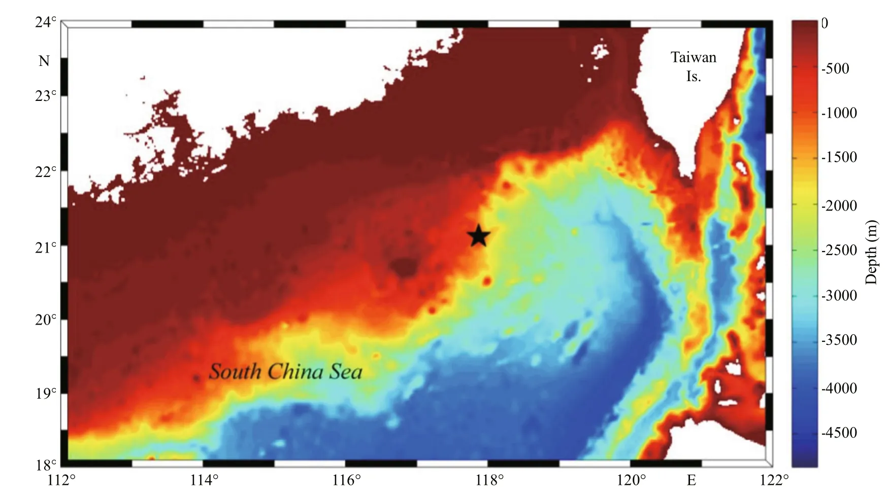
Fig.1　Map of the northern SCSThe mooring is denoted by the black star.

whereHnis the amplitude,gnis the phase, andωnis the frequency of the M2, S2, N2, and K2for semidiurnal coherent components and the K1, O1, P1, and Q1for diurnal coherent components. By subtracting the coherent components from the bandpass fi ltered current data, the incoherent components are obtained.

The coherent and incoherent semidiurnal signals are next projected onto barotropic and baroclinic modes:

Fig.2　Density (a), buoyancy frequency profi les (b), and vertical structures of baroclinic modes (c) for horizontal velocity in different seasons

wherecis the eigenspeed,Nis the buoyancy frequency,andhis the water depth. The buoyancy frequency can be calculated using temperature and salinity data from the World Ocean Atlas 2005 (WOA05). Using the Thomson-Haskell method (Thomson, 1950; Haskell,1953; Fliegel and Hunkins, 1975), the eigenvalue problem can be solved. As can be seen in Fig.2, the climatological stratifi cation profi les merely differ slightly from each other in the upper 200 m.Consequently, the baroclinic modes are computed with the buoyancy frequency averaged over the three seasons. Based on the least square method,Umcan be calculated from the time series of currents and baroclinic modes; thus, the tidal currents of each mode and the full-depth currents can be calculated according to Eq.2. Details of the method of reconstruction of the full-depth currents can be found in Cao et al. (2015).Because vertical gaps in the measurements might render the fi ts of higher modes unstable (Zhao et al.,2012), and because the semidiurnal tides at our site are dominated by lower modes (shown in Section 3), three modes are used for the reconstruction of the semidiurnal tidal currents. Further analysis of the seasonal variations of the semidiurnal ITs is based on these reconstructed currents.

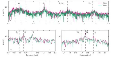
Fig.3　Power spectra of zonal velocity at depths of 200 and 800 m (a); details of the diurnal (b) and semidiurnal (c) constituents are shown in the lower panels

Regarding the diurnal signals, analysis of the modal content is performed in a qualitative manner,because the more complicated vertical structure of the diurnal component (Fig.8) poses a greater challenge for modal decomposition and current reconstruction.

3　RESULT AND DISCUSSION

3.1　Power spectra

Figure 3 shows the power spectra of zonal velocity during the entire study period at depths of 200 and 800 m, representative of the upper and bottom water column, respectively. At both depths, the spectra display the dominance of diurnal and semidiurnal constituents with additional peaks at overtides and compound tides (e.g., O1+M2and M4) implying a degree of nonlinearity to the IT fi eld. Closer inspection of the semidiurnal frequency band shows that tidal currents are much stronger in the upper layer. The O1tidal constituent within the diurnal band also displaysa pattern ofintensifi cation at the surface, while spectral peaks at the frequencies of K1and Q1are of similar magnitude, indicating strong currents in both the upper and the bottom layers.

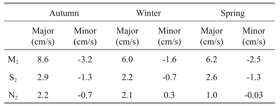
Table 1　Major and minor axes of semidiurnal tidal current ellipses

3.2　Semidiurnal tides

3.2.1Tidal current ellipses

The power spectra indicate dominance of the M2tide in the semidiurnal signal, which is further quantified by harmonic analysis. Tidal ellipse parameters of the principal semidiurnal constituents are calculated using the T-tide toolbox (Pawlowicz et al., 2002). Table 1 displays the major and minor axes of the tidal ellipses of the depth-averaged currents in different seasons. Despite seasonal changes, the M2tide is much stronger than the S2and N2throughout the entire observational period, i.e., the lengths ofits axes are at least twice as long as the other tides.Therefore, we investigate further the vertical structure of the M2elliptical features.

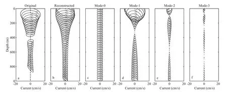
Fig.4　Vertical structures of original (a) and reconstructed (b) M2tidal ellipses as well as their corresponding modes (c)-(f)The ellipses are centered at their corresponding measurement depths and the dashed lines show their local phases at the start time.

The M2tidal currents in each season are fi rst extracted from the full-depth currents reconstructed using the method described in Section 2.2. The results for the winter segment are shown as an example. The absolute errors of the zonal and meridional velocities of the M2tide averaged both in depth and in time are 0.33 and 0.26 cm/s, respectively, indicating successful reconstruction. The reconstructed tidal ellipses are consistent with the observed tidal ellipse (Fig.4),showing that currents weaken as depth increases,which confi rms the conclusion based on the power spectra. The barotropic mode and the fi rst baroclinic mode dominate the M2tidal constituent, while higher modes play less important roles.

Following the same procedure, we can obtain vertical structures of the M2tide in different seasons(Fig.5). During the entire observational period, the M2tide maintains a similar vertical structure, i.e., both axes of the tidal ellipses reach their maxima in the upper 100 m, decrease rapidly with depth, and remain nearly constant below 400 m. Nevertheless, the M2tide does show seasonal variation. It is strongest in autumn and weakest in winter at all depths. To quantify this observation, the depth-integrated HKE averaged over one tidal cycle is computed as

whereu(z,t) andv(z,t) are the zonal and meridional velocities, respectively, and the angled brackets indicate the average over one tidal cycle. The calculation results are 3.97, 1.82, and 2.72 kJ/m2for autumn, winter, and spring, respectively. It can be found that a 180° transition of the local phase is clearer in autumn and spring, with the node of rapid change fl uctuating around the zero-crossing depth of the fi rst baroclinic mode, which implies a larger proportion of the fi rst-mode signal.

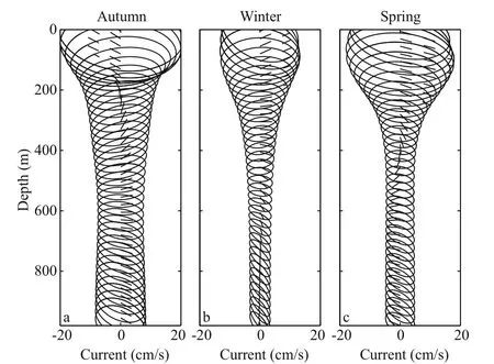
Fig.5　Vertical structures of the reconstructed M2tidal ellipses: (a) autumn, (b) winter, and (c) springThe ellipses are centered at their corresponding measurement depths and the dashed lines show their local phases at the start time.

3.2.2Coherent and incoherent features

Figure 6 illustrates time-depth graphs of the coherent and incoherent components of the semidiurnal currents. It is evident that the coherent component is apparently much stronger than the incoherent component. In the coherent component,the opposite currents in the shallow and deep waters imply the dominant role of the fi rst baroclinic mode.Conversely, the incoherent component shows multiple 180° transitions of phase in the vertical direction,which can be attributed to higher modes.

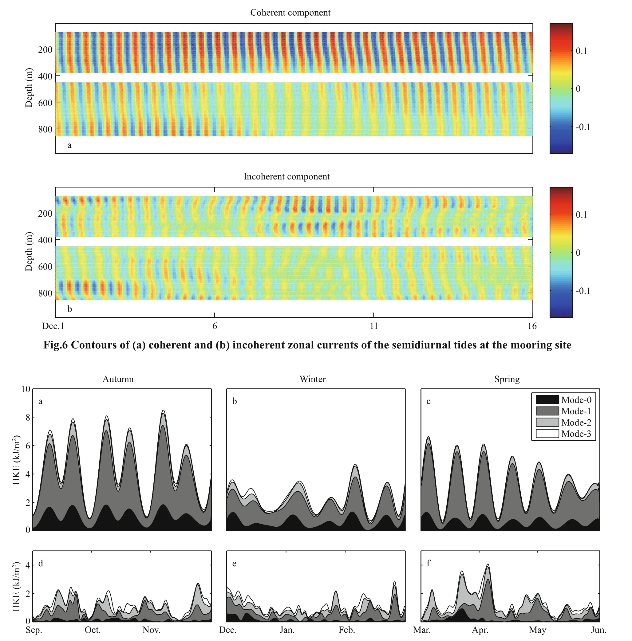
Fig.7　Depth-integrated HKE of semidiurnal (a)-(c) coherent and (d)-(f) incoherent components: (a) and (d) autumn, (b)and (e) winter, and (c) and (f) spring

Modal decomposition is performed for the coherent and incoherent components. To measure the contribution of each mode, the depth-integrated HKE is calculated. The HKE of the semidiurnal coherent and incoherent components are plotted as stacked bands colored by mode in Fig.7, and the detailed statistics are presented in Table 2. The modal decomposition results show that the fi rst mode dominates the coherent component with its proportion varying from 57% in winter to 72% in spring. It is followed by mode-0, i.e., the barotropic mode. Higher modes make only minimal contributions. The rises and falls of the barotropic and the baroclinic modes are generally in phase. However, the incoherent component has a different modal structure. The fi rst mode is slightly stronger than the second mode in terms of the seasonal average; however, the fi rst two modes sometimes show comparable magnitudes andthey even alternate in assuming the dominant role.Weak as it is, the third mode accounts for a larger proportion of the incoherent component than its counterpart does in the coherent component. The barotropic mode is weakest in the incoherent component. These results confi rm the preliminary conclusion drawn from Fig.6, i.e., for semidiurnal ITs at our site, the coherent component is dominated by the fi rst mode while the incoherent component is dominated by higher modes.

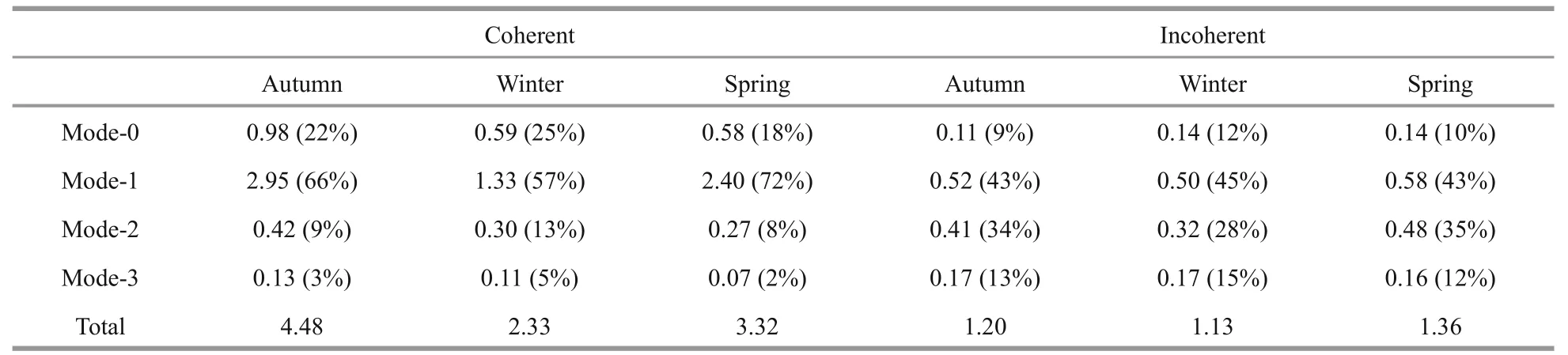
Table 2　Depth-integrated HKE averaged over one tidal period of each mode and its proportion in the semidiurnal coherent or incoherent components (Unit: kJ/m2)

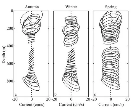
Fig.8　Vertical structures of the K1tidal ellipses: (a) autumn,(b) winter, and (c) springThe ellipses are centered at their corresponding measurement depths and the dashed lines show their local phases at the start time.

Overall, the coherent component is much stronger than the incoherent component; its proportion in the total HKE varies from 79% in autumn to 67% in winter. It has a regular 14-day spring-neap cycle,which is attributed to the modulation of the M2and S2tides. The coherent component varies with season; its HKE reaches a maximum of 4.48 kJ/m2in autumn and a minimum of 2.33 kJ/m2in winter. Conversely,the incoherent component shows little seasonal variation, which is consistent with its intermittent nature.

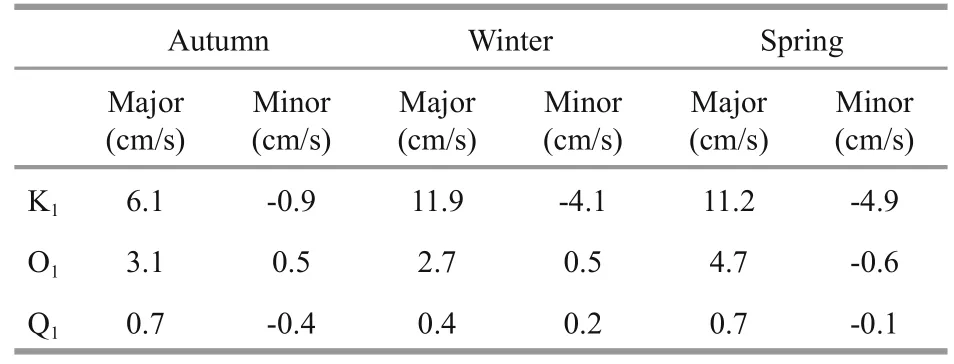
Table 3　Major and minor axes of diurnal tidal current ellipses

3.3　Diurnal tides

The continental slope of the northern SCS and the west ridge of the LS are supercritical to diurnal ITs,reflecting and trapping them within the SCS basin(Klymak et al., 2011; Wu et al., 2013). Diurnal tides with a complicated vertical structure contain higher modes, posing considerable challenges to current reconstruction, i.e., producing either unstable solutions for a large number of modes or less accurate solutions for lower modes (Zhao et al., 2012).Therefore, we analyze the characteristics of diurnal tides based on the original data and make a comparison with semidiurnal tides in a qualitative manner.

Harmonic analysis is fi rst conducted on the depthaveraged diurnal signals to identify the most important constituent(s). The major and minor axes of the principal diurnal constituents are shown in Table 3. It is evident that the K1tide dominates the others with both its axes being at least two times longer despite the seasonal changes. Consequently, the K1is selected for analysis of the vertical structure (Fig.8). Quite different from the M2, the K1tide has a more complicated vertical structure and clearer seasonal variation. In autumn, the K1tide intensifi es at depths of approximately 80, 200, and 850 m. It shows a similar vertical structure in winter except for weaker currents near the surface. In addition, currents in the middle of the water column are almost rectilinearly polarized in both autumn and winter. In spring, the K1tide becomes much stronger at all depths. The nearly constant amplitudes and phases in the vertical direction imply a dominant role of the barotropic mode.

Fig.9　Typical time-depth maps of (a), (c), and (e) coherent and (b), (d), and (f) incoherent diurnal signals(a) and (b) autumn, (c) and (d) winter, and (e) and (f) spring.

Coherent and incoherent features are also explored for diurnal signals. Figure 9 shows time-depth maps of zonal currents for a month representative of each season. Similar to those of the semidiurnal tides, the diurnal incoherent components show high wavenumber signals (e.g., the second mode around 16 September and the third mode around 31 December) and intermittent features. The barotropic signal accounts for a large proportion of the coherent component, except for autumn when it is dominated by the fi rst baroclinic mode. A difference in modal content between the coherent and incoherent components has been observed in the southern SCS(Liu et al., 2015). Because of modulation of the K1and O1tides, the coherent component has a 14-day spring-neap cycle, which is absent from the weaker incoherent constituents. Furthermore, the spring tide in the middle layer is not always in phase with those near the surface and the bottom, possibly due to the reflection of diurnal ITs.

To characterize the seasonal variation of diurnal tides, the depth-integrated HKE is computed as for semidiurnal tides but based on the original diurnal data (Fig.10). Similar to the semidiurnal currents, the coherent component accounts for a larger proportion of the total energy and it shows a regular 14-day spring-neap cycle, consistent with the conclusion drawn from Fig.9. However, its seasonal pattern is different to the semidiurnal coherent component, i.e.,stronger in winter than in the other seasons.

3.4　Discussion

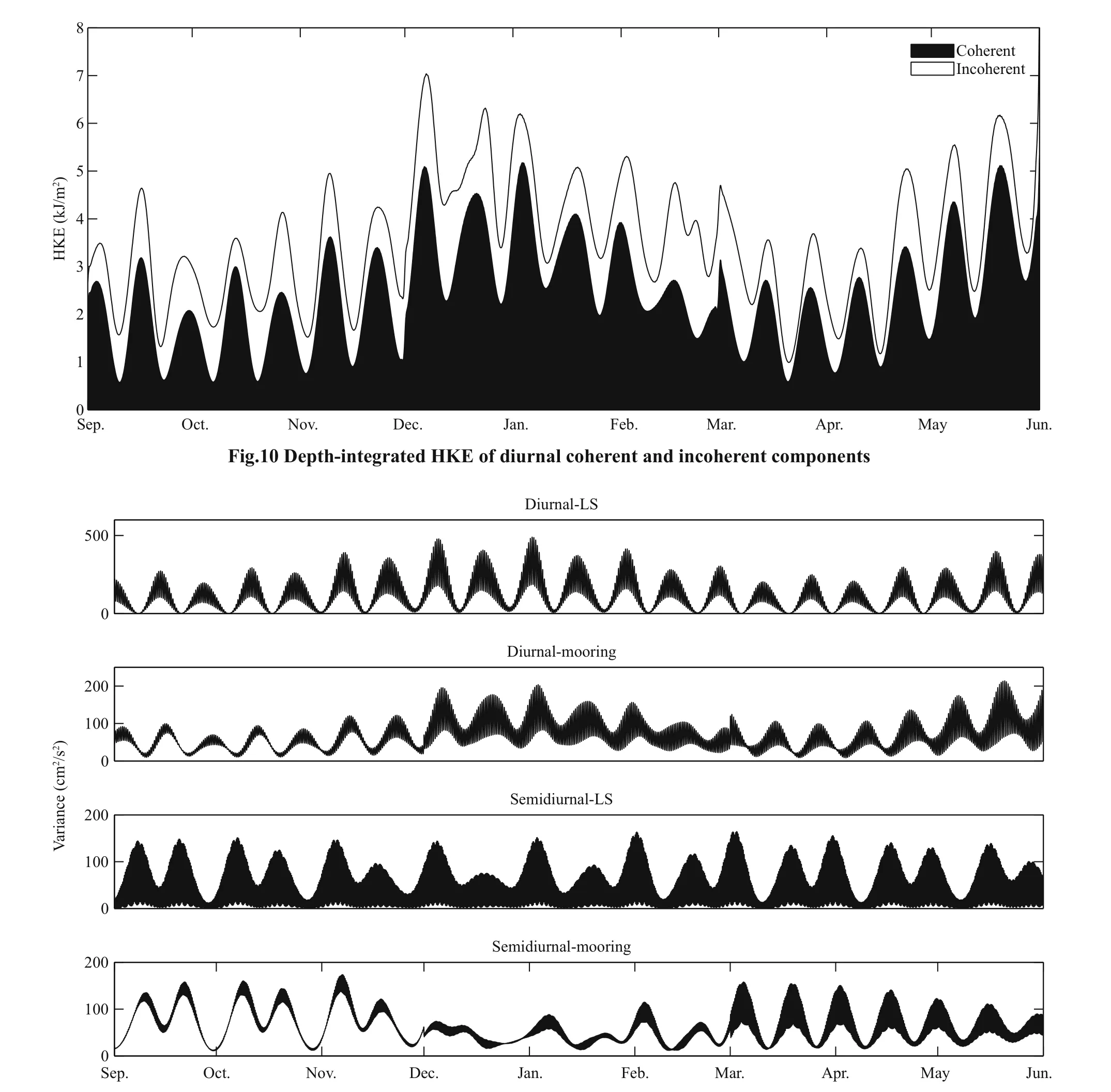
Fig.11　Barotropic current variances in the LS and vertically averaged coherent variances at the mooring for diurnal and semidiurnal frequency bands during the observation period

Diurnal and semidiurnal ITs on the edge of the SCS basin have different seasonal behaviors, as described above. Semidiurnal tides are weakest in winter when diurnal tides have the greatest energy. Numerical simulations and satellite observations have revealed that ITs in the northern SCS mainly originate from the LS and then propagate westward (Jan et al., 2008;Zhao, 2014). Therefore, it is natural to consider astronomical forcing within the LS for an explanation.Diurnal and semidiurnal barotropic current variances(Var=u2+v2) were derived from the Oregon State University Tidal Inversion Software (OTIS, Egbert and Erofeeva, 2002), predictions of which have been proven to agree well with in situ observations around the LS (Ramp et al., 2004; Alford et al., 2011). The variance was also computed for diurnal and semidiurnal coherent components at the mooring and averaged over the entire depth. As shown in Fig.11,the spring-neap cycle of coherent variances is generally in phase with the barotropic forcing in the LS. Furthermore, tidal currents show similar seasonal behaviors at the mooring and at the LS, i.e., the diurnal tides intensify in winter when the semidiurnal tides are weakest. These fi ndings imply that the temporal variation ofiTs can be attributed to astronomical forcing at the generation site. Previous studies have revealed that ITs in the deep basin to the west of the LS are mainly modulated by astronomical tides in the LS (Xu et al., 2014). However, ITs on the continental slope and shelf area of the SCS show seasonal patterns different from their astronomical forcing (Guo et al., 2012; Xu et al., 2013). This is explained by the interaction of the ITs with the seasonal thermocline (Xu et al., 2014). Our observations show that ITs on the western edge of the SCS basin maintain the seasonal behavior of their barotropic forcing in the LS. Furthermore, the observations on the continental shelfin those earlier studies were obtained from sites in shallower water to the west of ours. Therefore, we can conclude that it is in shallower water that the seasonal thermocline has an important effect on the seasonal behavior ofiTs.

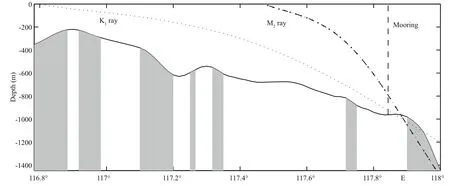
Fig.12　Bathymetry along 21.12°NSemidiurnal (M2) and diurnal (K1) IT characteristics are shown for reference. The region supercritical to the diurnal tide is indicated with gray shading.

Diurnal tides also differ from semidiurnal tides in terms of vertical structure, which we attribute to their reflection on the continental slope. Internal waves can transfer their energy to higher wavenumbers after critical reflection (Eriksen, 1982, 1985). Observations have confi rmed that the reflection of a mode-1 IT propagating onto the Virginia continental slope can give rise to a higher wavenumber response (Nash et al., 2004). As can be seen in Fig.12, the continental slope to the west to our observation site is supercritical with respect to diurnal tides but subcritical with respect to semidiurnal tides. reflection of diurnal tides has been observed by Klymak et al. (2011) at two moorings near our site. Therefore, reflection is a reasonable explanation for the higher mode signals at diurnal frequencies (Fig.9b, d, f).

4　SUMMARY

In this study, a nine-month mooring record was analyzed with the objective of characterizing the modal content and seasonal variation ofiTs on the edge of the SCS basin. Results show that coherent components of both diurnal and semidiurnal tides have clear seasonal variation and a regular 14-day spring-neap cycle, while incoherent components are more intermittent. They also differ from each other in terms of modal content, i.e., higher modes account for a larger proportion of the incoherent components.Differences exist between the semidiurnal and diurnal signals. The semidiurnal tides are weakest in winter when diurnal tides are strongest. Seasonal patterns ofiTs and barotropic tides within the LS, i.e., the generation site ofiTs, show good agreement. This implies that the seasonal behavior ofiTs is dictated by their astronomical forcing, even after extended propagation across the SCS basin, rather than by interaction with the thermocline. In terms of the vertical structure, the diurnal signals contain a greater number of higher modes, which is different from the domination of low modes in semidiurnal ITs. A reasonable explanation for this is reflection of the diurnal tide from the supercritical slope.

5　ACKNOWLEDGEMENT

The mooring data used this paper were obtained by the South China Sea Mooring Array constructed by the Ocean University of China. The authors deeply thank Professor TIAN Jiwei for providing the mooring data.