NUMERICAL SIMULATIONS FOR A VARIABLE ORDER FRACTIONAL CABLE EQUATION∗

A.M.NAGY

Department of Mathematics,Faculty of Science,Benha University,Benha 13518,Egypt

E-mail:abdelhameed nagy@yahoo.com

N.H.SWEILAM

Department of Mathematics,Faculty of Science,Cairo University,Giza 12613,Egypt

E-mail:nsweilam@sci.cu.edu.eg

1 Introduction

The cable equation has been recently treated by numerous of authors and is found to be a useful approach for modeling neuronal dynamics.The cable equation can be deduced from the Nernst-Planck equation for electrodiffusion in smooth homogeneous cylinders and it was investigated for modeling the anomalous diffusion in spiny neuronal dendrites.Henry et al[4]derived a fractional cable equation from the fractional Nernst-Planck equations to model anomalous electrodiffusion of ions in spiny dendrites which is similar to the traditional cable equation except that the order of derivative with respect to the time or space is fractional.

Fractional calculus is a mathematical branch investigating the properties of integrals and derivatives of non-integer orders.The applications of fractional calculus occur in several fields,such as physics,engineering, fluid flow,viscoelasticity,and control theory of dynamical systems(see[1,7,8,13,16,19,21–23]).The variable order calculus is a natural extension of the constant order(integer or fractional)calculus[24,25].The concepts of fractional differentiation and integration of variable order fractional are suggested by Samko and Ross in[20].There are several proposed definitions for the variable order fractional derivative definitions;for more details,see[5,6,9–11].In general,the variable-order fractional derivative is an extension of constant-order fractional derivative,where maybe the order function depends on one parameter,such as space or time,or system of other parameters[20,24].The variable order differentials have been studied in several applications such as control of a nonlinear viscoelasticity oscillator and the motion of particles suspended in a viscous fluid with drag force determined;for more details,see[17,18]and the references cited therein.

The main goal of this work is to solve variable order cable equation numerically by an accurate numerical method based on Crank-Nicolson method.In what follows,we give the definition of Riemann-Liouville variable order fractional derivatives and Grünwald-Letnikov variable order fractional derivatives,which will be used in our study.

Definition 1.1([17]) The Riemann-Liouville variable order fractional derivative is defined as

where n−1＜α(x)＜n.

Definition 1.2([14])The Grünwald-Letnikov variable order fractional derivative is defined as

where[x/h]means the integer part of x/h andare the normalized Grünwald weightswhich are defined by

The layout of this article is as follows:In Section 2,the variable order fractional cable equation is discretizated based on Crank-Nicolson method and shifted Grünwald formula;In Section 3,the stability analysis of the proposed method is discussed;In Section 4,linear and nonlinear numerical examples of variable order fractional cable problem are considered to show the accuracy of the scheme.Conclusions are given in Section 5.

2 Crank-Nicolson Scheme for Solving Variable Order Fractional Cable Equation

In this section,we combine two schemes Crank-Nicolson method and shifted Grünwald formula to solve the variable order fractional cable equation[2]on the form:

subject to

where 0 ＜ β(x,t),α(x,t)＜ 1,µ ＞ 0 is a constant andis the variable order fractional derivative defined by the Riemann-Liouville operator of order 1−γ(x,t),where γ(x,t)is equal to β(x,t)or α(x,t).

Before constructing the proposed scheme,let us consider the uniform grid points of the space and time are defined as follows:respectively,where M and N are integers such that h=L/N,τ=tmax/M.Equation(2.1)can be written at the grid points(xn,tm)as follows:

The Riemann-Liouville fractional partial derivative of order 1−γn,mcan be written using the Grünwald-Letnikov definition in the following form[15]:

The right-hand side of equation(2.4)can be approximated from[14]by

Consequently,Equation(2.4)leads to

It is well known that,the formula in the above equation is not always unique because of the fact there are numerous choices for the coefficientsthat lead to approximations of various orders p[12,14].The definition offor a first order accuracy(that is,p=1)is given by

Lemma 2.1([3])If,for n=1,2,···,N,m=1,2,···,M,l=0,1,···,the coefficientssatisfy:

and the Crank-Nicolson method is used to approximate the second derivative in the right hand side of Equation(2.1),that is,the average of the explicit scheme and the implicit scheme evaluated at the previous and current time steps respectively,then one gets

Also,if f(x,t)has first-order continuous derivative,then

Plugging Equations(2.7)–(2.9)into Equation(2.1),we have

Applying the Grünwald-Letnikov definition for fractional variable-order given in(2.6)to Equation(2.10),we obtain

where

After preforming some simplification,Equation(2.11)is written as

where C0,C1,···,Cm−2;A;B are matrices of order(N − 1)× (N − 1).The matrix A is a strictly diagonally dominant matrix

3 Stability Analysis

In this section,we analyze the stability analysis of the proposed scheme given in(2.14)for the free force case.

Theorem 3.1The Crank-Nicolson discretization with the shifted Grünwald estimation for the variable order fractional cable equation defined in(2.1)is unconditionally stable for 0＜ β(x,t)＜1 and 0＜ α(x,t)＜1.

ProofLet us define

then Equation(2.14)can be rewritten as If we assume as in the von Neumann stability procedure thatthen we obtain

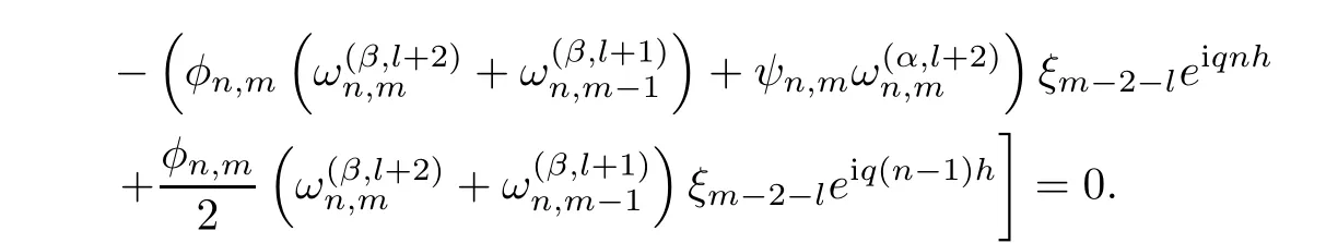
Divided by eiqnh

Suppose eiθ=cosθ+isin θ,then we obtain

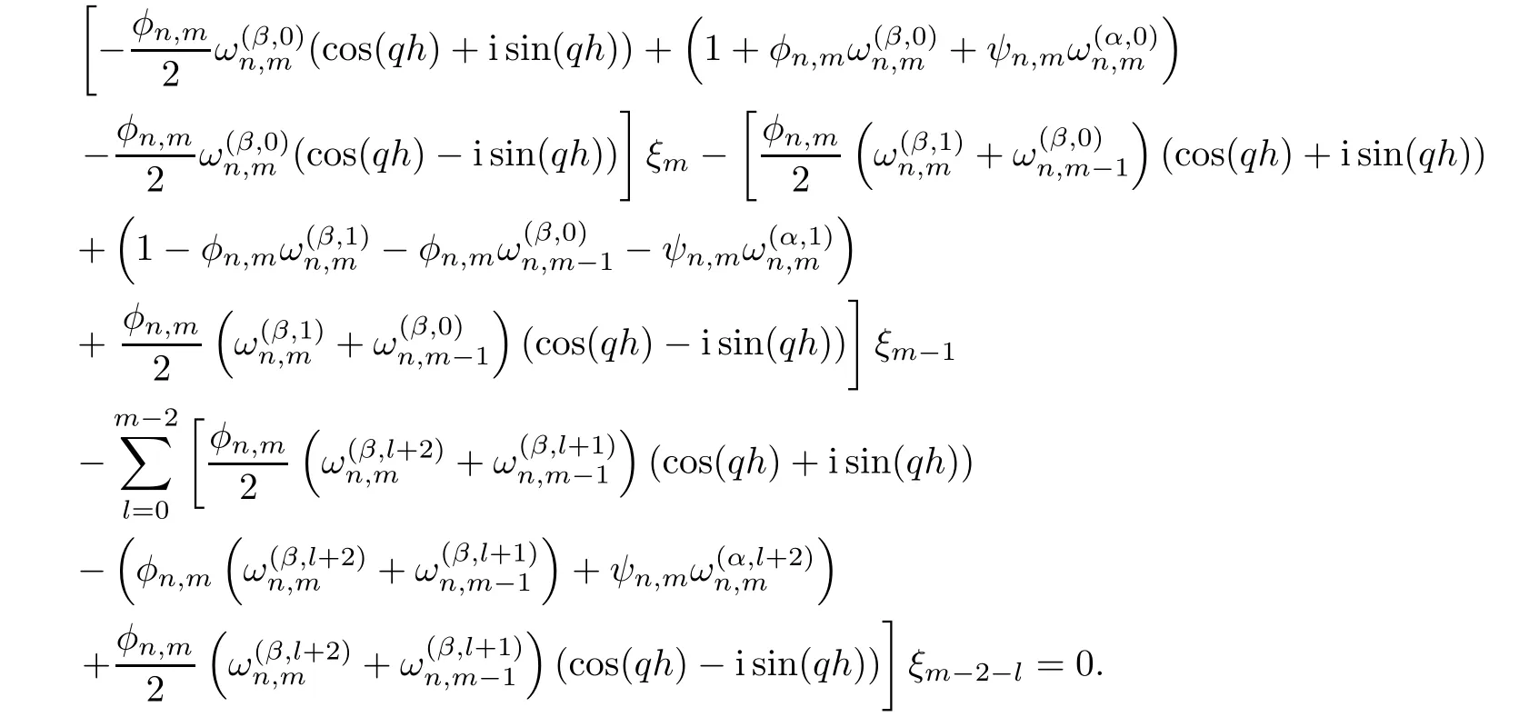
Simplifying the above equation,once we get

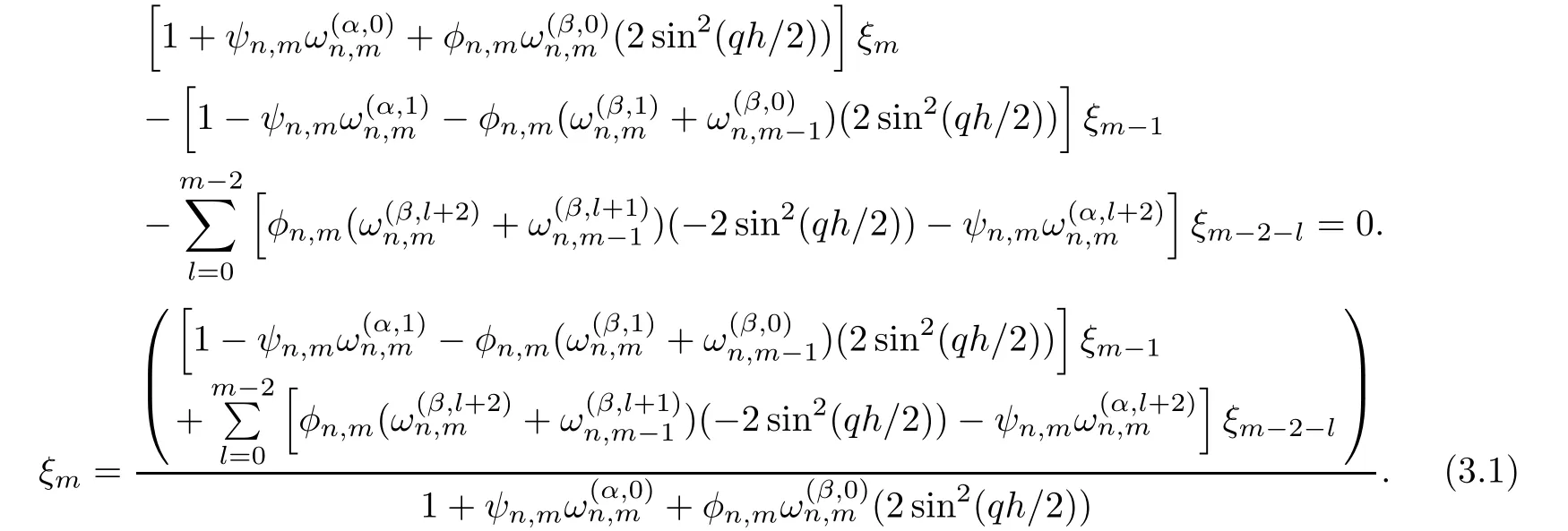
From Equation(3.1)and Lemma 2.1,becausefor all n,m,α,β,h and q,it follows that

and

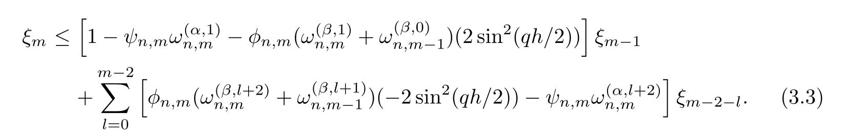
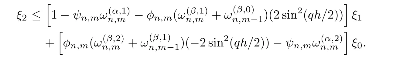
Thus,for n=2,the last inequality implies

Repeating the process until ξl≤ ξl−1,l=1,2,···,m − 1,we have

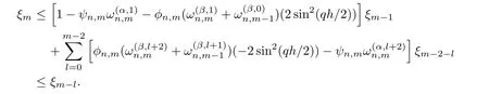
This shows that inequalities(3.2)and(3.3)imply that ξm≤ ξm−1≤ ξm−2≤ ···≤ ξ1≤ ξ0.Thus,which entailsand so the proposed scheme is unconditionally stable.

4 Numerical Experiments

In this section,we illustrate the applicability of the proposed technique discussed in the previous section for solving cable equation of linear and nonlinear variable-order fractional partial differential equations and compare our results with exact solutions.

Example 4.1Consider the following initial-boundary problem of the variable-order fractional cable equation

on a finite domain 0＜x＜1,with 0≤t≤tmax.

The source term is given by

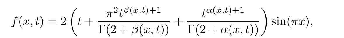
the initial and boundary conditions are u(x,0)=0;u(0,t)=u(1,t)=0,and the exact solution is u(x,t)=t2sin(πx).

In Table 1,we list the maximum absolute errors between exact and approximate solutions using the proposed approach with different choices of constant values of α and β.Moreover,Table 2 shows the maximum absolute errors at t=1,using different values of β(x,t)and α(x,t).

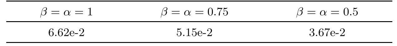
Table 1 The maximum absolute error of the proposed approach using different values of constant β and α at N=10 and M=15

Table 2 The maximum absolute error of the proposed approach using different values of β(x,t)and α(x,t)

Figures 1,3,5 and 7 show the graphs of exact and numerical solutions of the proposed approach at t=1,with various values of α(x,t), β(x,t)and τ,h.Moreover,Figures 2,4,6 and 8 show 3D-drawing of the absolute error of exact and approximate solutions with different values of α(x,t), β(x,t)and τ,h.From the results presented in Tables 1,2 and all figures,it is clear that the proposed approach provides accurate numerical solutions coincide closely with the exact solutions.

Example 4.2Consider the following initial-boundary problem of the variable-order fractional nonlinear cable equation,

on a finite domain 0＜x＜1,with 0≤t≤tmax.The source term is given by

the initial and boundary conditions are u(x,0)=0;u(0,t)=t2and u(1,t)=et2,and the exact solution is u(x,t)=ext2.

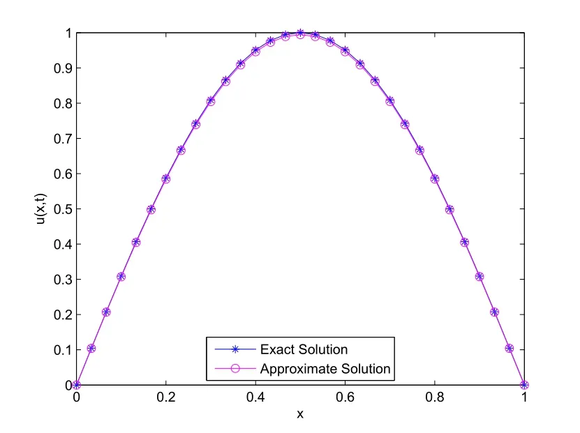
Figure 1 The behavior of the numerical and exact solutions at β(x,t)=5xt−3,α(x,t)=and τ=h=1/30

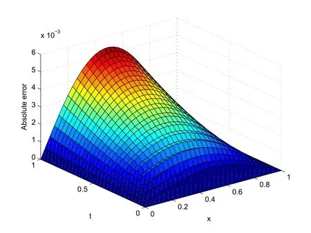
Figure 2 The graph of the absolute error at β(x,t)=5xt−3,α(x,t)=and τ=h=1/30 for Example 4.1

Figure 3 The behavior of the numerical and exact solutions at β(x,t)=5xt−3,α(x,t)=,and τ=h=1/50

Figure 4 The graph of the absolute error at β(x,t)=5xt−3,α(x,t)=and τ=h=1/50 for Example 4.1.

Figure 5 The behavior of the numerical and exact solutions at β(x,t)=α(x,t)=and τ=h=1/30

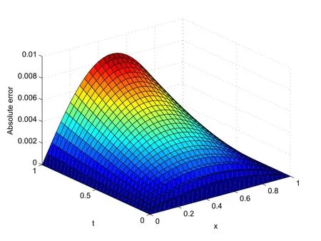
Figure 6 The graph of the absolute error at β(x,t)=and τ=h=1/30 for Example 4.1

Table 3 shows the maximum absolute error for Example 4.2 at different values of β(x,t),α(x,t),N and M.The graphs of the absolute error between the exact and the approximate solutions forτ=h=1/30 are shown in Figures 9 and 10,respectively.

Table 3 The maximum absolute error of the proposed approach using different values of β(x,t)and α(x,t)

Figure 7 The behavior of the numerical and exact solutions at β(x,t)=α(x,t)=and τ=h=1/50

Figure 8 The graph of the absolute error at β(x,t)=and τ=h=1/50 for Example 4.1

Figure 10 The graph of the absolute error at β(x,t)=and τ=h=1/30 for Example 4.2

Figure 9 The graph of the absolute error at β(x,t)=and τ=h=1/30 for Example 4.2

5 Conclusions

In this article,we have presented a new technique for solving the variable-order cable equation.The proposed technique is based on Crank-Nicolson method with shifted Grünwald estimation for variable-order fractional derivatives.Special attention is given to discuss the stability of the proposed technique.Finally,some numerical examples are given to clarify the validity and accuracy of the proposed technique.The obtained numerical results are compared with exact solutions.The numerical results show that the proposed technique is accurate for solving such type of fractional differential equations.All numerical computations were performed in MATLAB software version R2012a.

[1]Benson A D,Wheatcraft W S,Meerschaert M M.The fractional-order governing equation of Lévy motion.Water Resour Res,2000,36(6):1413–1424

[2]Chang C M,Liu F,Burrage K.Numerical analysis for a variable-order nonlinear cable equation.J Comput Appl Math,2011,236(2):209–224

[3]Chen Chang-Ming,Liu F,Anh V,Turner I.Numerical schemes with high spatial accuracy for a variableorder anomalous subdiffusion equation.SIAM J Sci Comput,2010,32(4):1740–1760

[4]Henry I B,Langlands M A T,Wearne L S.Fractional cable models for spiny neuronal dendrites.Phys Rev Lett,2008,100:128103pp

[5]Ingman D,Suzdalnitsky J.Control of damping oscillations by fractional differential operator with timedependent order.Comput Methods Appl Mech Eng,2004,193(52):5585–5595

[6]Ingman D,Suzdalnitsky J,Zeifman M.Constitutive dynamic-order model for nonlinear contact phenomena.J Appl Mech,2000,67(2):383–390

[7]Kilbas A A,Srivastava M H,Trujillo J J.Theory and applications of fractional differential equations.San Diego:Elsevier,2006

[8]Langlands M A T,Henry I B,Wearne L S.Fractional cable equation models for anomalous electrodiffusion in nerve cells:in finite domain solutions.J Math Biol,2009,59(6):761–808

[9]Liu F,Zhuang P,Anh V,Turner I.A fractional-order implicit difference approximation for the space-time fractional diffusion equation.ANZIAM J,2006,47:C48–684

[10]Lorenzo C F,Hartley T T.Variable order and distributed order fractional operators.Nonlinear Dyn,2002,29:57–98

[11]Lorenzo C F,Hartley T T.Initialized fractional calculus.Internat J Appl Math,2000,3(3):249–265

[12]Lubich C.Discretized fractional calculus.SIAM J Math Anal,1986,17:704–719

[13]Nagy A M,Sweilam N H.An efficient method for solving fractional Hodgkin-Huxley model.Phys Lett A,2014,378:1980–1984

[14]Podlubny I.Fractional differential equations.San Diego:Academic Press,1999

[15]Podlubny I,El-Sayed A M A.On two definitions of fractional derivatives.Slovak Academy of Sciences,Institute of Experimental Physics,1996:ISBN 80-7099-252-2

[16]Quintana-Murillo J,Yuste B S.An explicit numerical method for the fractional cable equation.Int J Differential Equations,2011,2011:12pp

[17]Ramirez L E S,Coimbra C F M.On the selection and Meaning of variable order operators for dynamic modeling.Int J Differ Equat,2010,2010:16pp

[18]Ramirez L E S,Coimbra C F M.A variable order constitutive relation for viscoelasticity.Ann Phys,2007,16(7/8):543–552

[19]Reynolds A.On the anomalous diffusion characteristics of membrane bound proteins.Phys Lett A,2005,342:439–442

[20]Samko S G,Ross B.Integration and differentiation to a variable fractional order.Integral Transforms Spec Funct,1993,1(4):277–300

[21]Sweilam N H,Khader M M,Nagy A M.Numerical solution of two-sided space-fractional wave equation using finite difference method.J Comput Appl Math,2011,235(8):2832–2841

[22]Sweilam N H,Nagy A M.Numerical solution of fractional wave equation using Crank-Nicolson method.World Appl Sci J,2011,13(Special Issue of Applied Math):71–75

[23]Sweilam N H,Nagy A M,El-Sayed Adel A.Second kind shifted Chebyshev polynomials for solving space fractional order diffusion equation.Chaos Solitons Fractals,2015,73:141–147

[24]Sweilam N H,Nagy A M,Assiri T A,Ali N Y.Numerical simulations for variable-order fractional nonlinear differential delay equations.J Fract Calc Appl,2015,6(1):71–82

[25]Sweilam N H,Assiri T A.Numerical simulations for the space-time variable order nonlinear fractional wave equation.J Appl Math,2013,2013:7pp