STABILITY AND BIFURCATION ANALYSIS OF ADELAYED INNOVATION DIFFUSION MODEL∗

Rakesh KUMAR

Department of Applied Sciences,S.B.S.State Technical Campus,Ferozepur,Punjab 152004,India;Research Scholar with I.K.G.Punjab Technical University,Kapurthala,Punjab 144603,India

E-mail:keshav20070@gmail.com

Anuj Kumar SHARMA

Department of Mathematics,L.R.D.A.V.College,Jagraon,Ludhiana,Punjab 142026,India

E-mail:anujsumati@gmail.com

Kulbhushan AGNIHOTRI

Department of Applied Sciences,S.B.S.State Technical Campus,Ferozepur,Punjab 152004,India

E-mail:agnihotri69@gmail.com

1 Introduction

Articles[1,2],and in particular[3],represented the starting point of a stream concerning the study of the time path of the spread of new consumer durables over a population of potential consumers.The first marketing innovation diffusion model was proposed by Bass,and it is still providing the foundation for developing the new hypotheses for gaining insight into the diffusion and penetration of innovations among the potential adopters.In the Bass model,the market m is assumed to be fixed,and the evolution of the adopters is described by

Where A(t)is the number of adopters at time t;The parameter p takes into account new adopters who join the market as a result of external in fluences such as activities of firms in the market,advertising,attractiveness of the innovation;The parameter q is the coefficient of imitation and refers to the rate of in fluence of adopters on nonadopters.

The model has been widely used to understand the spread of new products and to understand the underlying phenomena responsible for the diffusion of new technology(market innovation)or new products in the market[4–13].According to Rogers[14],“a technological innovation is a design for instrumental action that reduces the uncertainty in the cause-effect relationships involved in achieving the desired outcome.”The literature on mathematical modeling of innovation diffusion has accounted for a large number of contributions with different directions of investigation since the early 1960s.Rogers summarized his previous research in his book and concluded that the diffusion of innovations consists of five steps:awareness(individual is exposed to innovation),interest(individual seeks more information),evaluation(individual applies innovation to his or her situation),trial(individual uses innovation on a small scale),and adoption(individual makes full use of the innovation)[14].Furthermore,through the behavior research,he found that the five steps innovation diffusion processes can be simplified into two-step flow process,that is,media in fluences innovative opinion leaders to adopt a new product,who in turn force other people to adopt the product as well[14–18].Mahajan et al[16]discussed all the earlier contributions of the management and marketing literature to the cumulative understanding of the innovation diffusion dynamics.

The models with a time delay have been proposed by many researchers which exhibits the evaluation stage of a product[19–22].A mathematical model is intended to describe the dynamics of users of one product in two different patches[23].Stability of competitive innovation diffusion model in a market is explained in[24,25].Global stability of an innovation diffusion model for n products is discussed in[26].An innovation diffusion model with the nonlinear acceptance is reviewed to describe the dynamics of three competing products in a market[27].A binomial innovation diffusion model for a variable size market for demographic processes of entrance-exit from each market compartment was studied by F.Centrone[28].Another model with time delay is developed to consider the evaluation stage.Shukla et al proposed that innovation diffusion process is affected by variable external in fluences such as advertisements as well as the change of density of nonadopters population because of intrinsic growth rate,emigration or death rate,etc.The model analysis shows that the adopter’s population density increases as the parameters related to the growth rate of nonadopters population as well as the rate of external in fluences increase.The main effect of increasing density of variable external forces is to make the equilibrium level of adopters population density reach to its equilibrium with a much faster rate[29].Wang et al[22]have considered the aspect of delay in their studies to describe the process of evaluation and decision-making whereas Shukla et al explained that the innovation diffusion process is affected by variable external in fluences such as advertisements as well as change of density of non-adopters population because of intrinsic growth rate,emi-gration or death rate,etc.The studies on the diffusion of innovations are now challenging and essential issues from a marketing point of view for various companies/industries.Remarkably few studies have been performed in this direction,and to the best of our knowledge,no attention has been paid so far to consider logistically growing non-adopters population together with evaluation period(time delay).In this article,we propose an innovation diffusion model by taking into consideration the various demographic processes together with the evaluation period(time delay)to describe the process of diffusion of an innovation/technology.We aim to present a mathematical analysis of the conditions for the existence of Hopf bifurcation and analyze how the properties of the periodic solutions occur.In this model,we extend the work of Wang et al model by taking into consideration the logistically growing non-adopters immature population class,mature population class,and the adopter class,together with variable external as well as internal in fluences.The external forces for the adoption of an innovation lead us to consider the effect of media inclusive of electronic and print as well.The internal forces are a growth factor of the number of adopters and the interpersonal communication between who is already adopter and who is a potential adopter.With a time delay,we include the evaluation stage and the decision-making stage in the system.The innovation diffusion patterns identified by the theory of stability analysis and Hopf bifurcation are qualitative.Most frequently,the Hopf bifurcation theory is being used to classify diffusion patterns which are used for design or forecasting the future trends.

This article is organized as follows:In the next section,we will formulate the mathematical model consisting of a system of delay differential equation.Section 3 deals with some preliminaries,such as the positivity of solutions.The existence of various equilibria and formation of characteristic equation is given in Section 4.Section 5 deals with the asymptotical stability analysis of multiple equilibria.The study of the delayed innovation diffusion model,the particularly Hopf bifurcation analysis is investigated in Section 6.The subsequent section is devoted to determining the direction of the Hopf bifurcation and the stability of bifurcating periodic solutions by using normal form theory and the center manifold theorem in Section 7.Numerical simulations supporting the theoretical analysis are given in Section 8.This article ends with a conclusion and discussion in the last section.

2 Mathematical Model

In this article,we consider a delayed innovation diffusion model with stage structure and nonlinear incidence rate.We assume that only mature population can become the member of adopter population.We divide the population into three classes,namely,N1(t);N2(t);A(t),where N1(t)represents non-adopter population densities of the immature stage at time t,N2(t)is the non-adopter mature population,and A(t)is the adopter population class.To make the model more realistic,we involve various demographic structure of a population into the basic Bass model and the models proposed by[22,29].Furthermore,we are making the following assumptions for the formulation of our model system.

•The non-adopter immature population N1is following logistic growth with intrinsic rate r and carrying capacity K.Assume that δ is the emigration rate or death rate of the immature population.Also,the immature population is becoming the member of the mature population at the rate ω.It is assumed that only non-adopter mature population N2may become the member of adopter population class A.

•Suppose that p is the cumulative density of variable external factors,q is the cumulative density of variable internal factors,which is supposed to be constant.

•Assume that ε is the rate of adopters going back to mature nonadopter population class N2,who may become the member of adopter population class later on and η is the rate by which adopters discontinue to use the product forever.Assume thatµis the emigration rate or death rate of the nonadopter population class N2and adopter population class A.

• The variable external(advertisements),as well as internal(world of mouths)factors,affect the individual’s decision.Therefore,the rate of change of adopters is because of external as well as internal in fluences,their natural deaths,emigration rate,their rate of discontinuance to use the product.

•It is also assumed that shifting of non-adopter mature population N2to adopter population A is not instantaneous,that is,population N2take some evaluation period τ to evaluate the positive-negative of the innovation(product).It is clear that non-adopter enter into the adopter class only after going through the evaluation stage(that is,each non-adopter of the system take average evaluation time τ to evaluate the product).In particular,if an individual has information of the product at time t−τ,he may leave the evaluation class in the interval[t− τ,t]due to the death or since he gets uninterested in the product.

• The survival probability of an individual through the evaluation stage is e−µτ.Also,if ε is the rate that individuals leave the evaluation stage since they have decided not to buy the product,then e−ετis the fraction that individuals are still interested in the product at the end of the test period.Therefore,the success probability through the evaluation stage,that is,the probability that an individual who is aware of the product at time t− τ does not die and remains interested in the product at time t,is e−(µ+ε)τ.

•From a practical point of view,we consider saturation incidence rate in this research article,which is following Holling II type mutual interactions in between potential adopters and adopters.The rate of awareness at time t−τ with the help of variable internal in fluences isand we assume the force of adoption in this version iswhich is saturated with the adopter population.¯τ is the average time of evaluation,during which the nonadopter population evaluate the innovation and decides whether to adopt it or not.

•We suppose that the individuals who pass the evaluation stage will move to the adopter population class.Hence,because of the variable internal in fluences,is the number of individuals who will eventually be the members of adopter population.It is the rate of transfer of individuals who got knowledge(information)about the particular innovation at time t−τ because of variable internal in fluences and decided to be the member of adopter class at time t.Also,the rate of transfer with variable external in fluences from the non-adopter mature population N2to adopter population A at time t is pN2.

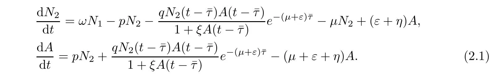
In this model,it is assumed that all the parameters are positive constants.In the light of the above mentioned modifications in the model proposed by Wang et al[22],the governing eqns.of our proposed model are given by(2.1):

3 Positivity of Solutions

We denote the Banach space of continuous functions

with the norm

by C,where ϕ =(ϕ1,ϕ2,ϕ3).Furthermore,let

The initial conditions for system(2.2)are

where ϕ =(ϕ1,ϕ2,ϕ3).It is well-known,by the fundamental theory of functional differential equations[30],that system(2.2)has a unique solution(n1(t),n2(t),a(t))satisfying the above initial conditions.It is easy to show that all solutions of system(2.2)corresponding to initial conditions are defined on[0,+∞)and remain positive for all t≥0.

In this section,we are trying to find the conditions that system(2.2)is positive.

Lemma 3.1All solutions of system(2.2)with initial conditions(3.1)are positive.

ProofWe prove the positivity by contradiction.Suppose that n1(t)is not always positive.Then,let t0＞0 be the first time such that n1(t0)=0.From the first equation of(2.2),we have˙n1(t0)=s＞0.By our assumption,this means n1(t)＜0,for t∈(t0−∈,t0),where∈is an arbitrary small positive constant.Implying that exist t′0＜ t0such that T(t′0)=0,this is a contradiction because we take t0as the first value at which T(t0)=0.It follows that T(t)is always positive.We now show that n2(t)＞0 for all t＞0.Otherwise,if it is not valid,nothing that n2(0)＞ 0 and n2(t)＞ 0,(−τ≤ t≤ 0),then there exist a t1such that n2(t1)=0.Assume that t1is the first time such that n2(t1)=0,that is,t1=inf{t＞0:n2(t)=0}.Then,t1＞0,and from system(2.2)with(3.1),we get

Thus,˙n2(t1)＞0.Thus,for sufficiently small∈＞0,˙n2(t1−∈)＞0.But by the definition of t1,˙n2(t1−∈)≤0.Again this is a contradiction.Therefore,I(t)＞0 for all t.In the same way,we see that a(t)is always positive.Thus,we can conclude that all solutions of system(2.2)with(3.1)remain positive for all t＞0.

4 Equilibrium Points

4.1 Existence of equilibria

Irrespective of the parameter values,the DDE system(2.2)possesses three feasible equilibrium points on the boundary of:

(i)E0(0,0,0)is the trivial equilibrium;

(ii)E1(n1,n2,0)is the adopter free equilibrium,whereandIt is easy to check that E1is positive provided r＞ω+δ.

(iii)The nonnegative equilibriumwhere

and a∗are the roots of the equation

where Φ1=hb1m(βγ−αψ)+αb1(βγ−αψ)e−φτ+b1mβ(αζ−hγ),Φ2=cm(b−1)(αζ−hγ)+hb1(βγ−αψ)+chmγ(b−1)+cαγ(b−1)e−φτ+b1β(αζ−hγ),and Φ3=c(b−1)(αζ−hγ)+chγ(b−1).

It is quite difficult to find out exact unique interior equilibrium point in parametric form required for further investigation.But looking at the relative positions of nullcline,we can easily visualize the existence of positive equilibrium point(see Figure 1).This shows that the positive equilibrium point E∗exists for m=1.

Figure 1 Existence of a∗for m=1

4.2 Characteristic equation

where I is the identity matrix and

5 Stability of Equilibria

In this section,we will observe the stability of all equilibria of the model system(2.2).

5.1 Stability of equilibrium E0

For the trivial equilibrium E0(0,0,0),characteristic equation(4.2)becomes

Hence,E0is locally asymptotically stable provided if r＜ ω+δ and hψ ＞ βζ hold,that is,intrinsic growth rate of the non-adopter immature population is less than the total of their rate of shifting from immature to mature non-adopter population class and emigration rate/death rate of the immature population which is apparent condition for the existence of zero level of immature population of the system.

5.2 Stability of equilibrium E1

For the adopter free equilibrium E1(n1,n2,0),(4.2)is reduced to

Now,at E1(n1,n2,0),the first factor f1(λ)=b− 1 − 2b1= −(b−1)＜ 0 for r＞ ω+δ.and the roots of the second factor is negative,that is,f2(λ) ＜ 0 if γn2e−(φ+λ)τ＜ h+ ψ,and(hγ +αζ)e−φτ＜ hψ +βζ.Consequently,E1is locally asymptotically stable if r＞ ω +δ,h+ψ ＞ γn2e−(φ+λ)τ,and hψ +βζ＞ (hγ +αζ)e−φτhold.

Theorem 5.1The sufficient conditions for the local asymptotical stability for E1are as follows:

(1)r＞ω+δ;

(2)h+ ψ ＞ γn2e−(φ+λ)τ;

(3)hψ +βζ＞ (hγ +αζ)e−φτ.

The condition(1)in the above theorem is self explanatory and follows that instability of trivial equilibrium E0leads to stability of E1.

5.3 Stability at the equilibrium E∗

In this section,we shall discuss the stability of equilibrium point E∗of system(2.2).

At positive equilibrium E∗,(4.2)is reduced to the following equation

where

and the coefficients are given as follows:

For τ=0,the characteristic equation(5.2)becomes

where T1=A1(0)+B1(0),T2=A2(0)+B2(0),and T3=A3(0)+B3(0).

Using Routh-Hurwitz stability criterion for a characteristic polynomial of a three-dimensional system as in[31],that is,all the roots of equation(5.3)are negative if T1＞0,T2＞0 and T3＞0 and also T1T2−T3＞0.By making simple calculation,we see that all these conditions holds good only if

Hence,we may have the following lemma.

Lemma 5.2For τ=0,the positive equilibrium E∗of(2.2)is locally asymptotically stable if and only if(H∗):α ＞

6 Analysis of the Delayed Model

In this section,we will be happy to make stability analysis of system(2.2)with time delay τ around E∗.Here,we shall provide some analytical results and verification of these will be done in the section of numerical simulation.

Here,we investigate the existence of purely imaginary roots λ =iω (ω ＞ 0)of equation(5.2).

To see the instability caused by time delay τ,assume that for some τ＞ 0,λ =iω (ω ＞ 0,is a purely imaginary root of the characteristic equation(5.2).Then,by putting λ =iω into(5.2)and using the process followed by[32,33]to separate real and imaginary parts of the characteristic equation,we have

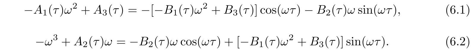
On solving(6.1)and(6.2),we get the following equation in ω

where

Set z=ω2,then we have

Set

Hence,the equation

has two roots

Now,we state the lemma proved by[34].

Lemma 6.1For the polynomial equation(6.4),we have the following results:

(i)If l3＜0,then(6.4)has at least one positive root;

(ii)If l3≥0,and Δ=−3l2≤0,then(6.4)has no positive root;

(iii)If l3≥0,and Δ=−3l2＞0,then(6.4)have positive roots if and only if=

Again for τ=0,(5.3)can be written as

Applying Lemma(6.1)to(6.8),we obtain the following lemma.

Lemma 6.2([35]) For the transcendental equation(5.2),we have the following results:

(i)If l3≥0 and Δ=−3l2≤0,then all roots with positive real parts of equation(5.2)has the same sum as those of the polynomial equation(6.8)for all τ≥0.

(ii)If l3＜0 or l3≥0,and0 and h′(z∗)≤0,then all roots with positive real parts of equation(5.2)has the same sum as those of the polynomial equation(6.8)for all τ∈ [0,τ∗).

With the help of Lemma 6.1 and Lemma 6.2,we can obtain the following lemma.

Lemma 6.3([36,37]) (i)The positive equilibrium E∗of system(2.2)is absolutely stable if and only if the equilibrium E∗of the corresponding ordinary differential equation system is asymptotically stable and the characteristic equation(5.2)has no purely imaginary roots for any τ＞ 0.

(ii)The positive equilibrium E∗of system(2.2)is conditionally stable if and only if all the roots of the characteristic equation(5.2)have negative real parts at τ=0 and there exists some positive value of τ such that the characteristic equation(5.2)has a pair of purely imaginary roots±iω.

ProofThe positive equilibrium point is asymptotically stable if all solutions of D(λ,τ)have negative real parts.As stated above,all solutions of D(λ,τ)have negative real parts at τ=0 if(H∗)hold.So,we assume that the condition(H∗)is satisfied.From the continuity of the solutions λ(τ)of D(λ,τ),equation(5.2)can have solutions with positive real parts if and only if D(λ,τ)has solutions with zero real parts for some τ＞ 0,that is,there exists purely imaginary solutions of equation(5.2). □

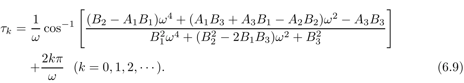
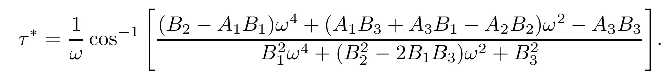
To determine how time delay affects the stability properties of interior equilibrium point,we shall consider τ as the bifurcation parameter,that is,and we are to check the instability caused in the system by time delay τ.Assume that for some τ＞ 0,iω is a purely imaginary characteristic root of(5.2).Therefore by using λ =iω into(5.2),we will be able to find the corresponding value of τ∗such that the characteristic equation(5.2)has a pair of imaginary roots given by

By Lemma(6.1),there exists at least one positive root ω =ω∗of equation(6.3)if l3＜0.By this condition,the characteristic equation(5.2)will have a complex conjugate pair of purely imaginary roots of the form ±iω,and a Hopf bifurcation might exist.

Let us now investigate whether model system(2.2)undergoes a Hopf bifurcation phenomenon atwhen τ increases through τ∗.From the theory of Hopf bifurcations[38,39],there are two conditions for the existence of a Hopf bifurcation:

(i)A purely imaginary complex conjugate pair of eigenvalues ±iω0exists with the real parts of all other eigenvalues being negative;

(ii)The transversality condition is satisfied.We have proved the first condition in Lemma 6.3.

To check the transversality condition for the occurrence of Hopf-bifurcation,we need to show that/=0 at σ =0.Taking λ(τ)= σ(τ)+iω(τ)in(5.2),and taking derivative w.r.t. τ,separating real and imaginary parts,setting τ= τ∗,σ =0 and ω = ω∗,we may obtain

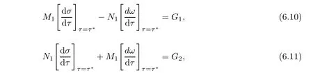
where

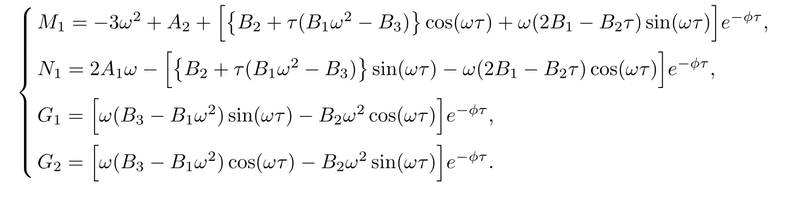
Solving(6.10)and(6.11),we get

But from this expression,it is quite difficult to assess whether the transversality condition is satisfied or not.We shall verify it numerically in the numerical simulation section.Hence,the conditions for Hopf bifurcation[40]are then satisfied at τ= τ∗which is the least positive value of τ given by(6.9).The stability of the zero solution of system(2.2)depends on the locations of the roots of the characteristic equation(5.2).When all roots of(5.2)locate in the left half of complex plane,the trivial solution is stable;otherwise,it is unstable.To investigate the distribution of roots of the transcendental equation(5.2),the following lemma is helpful.

Lemma 6.4(Ruan and Wei[41]) For the transcendental equation

as(τ1,τ2,τ3,···,τm)vary,the sum of orders of the zeroes of

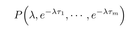
in the open right half-plane can change,and one zero appears only on or crosses the imaginary axis.

On the basis of the above analysis of hopf bifurcation and Lemma 6.4,we may state the following theorem.

Theorem 6.5([42]) Suppose that E∗exists and the conditions in(H∗)are satisfied for system(2.2),then the necessary and sufficient conditions for E∗to be locally asymptotically stable in the presence of an evaluation period τ are as follows:

(i)if τ∈ [0,τ∗),the positive equilibrium E∗is LAS;

(ii)if τ＞ τ∗,the positive equilibrium E∗is unstable;

(iii)at τ= τ∗,system(2.2)undergoes hopf-bifurcation around E∗,that is,as τ increases through τ∗,E∗bifurcates into small periodic solutions,where τ∗= τkfor k=0 is given by

7 Stability of Periodic Solutions

In the previous section,we obtain the conditions under which a family of periodic solutions bifurcates from the positive equilibrium at the critical value τ∗.In this section,it is interesting to determine the direction,stability,and period of the periodic solutions bifurcating from the positive equilibriumat the critical value τ∗by applying the normal form theory and the center manifold theorem as used by Hassard et al[40].Here,we will use the method of computing normal forms for FDEs introduced by Faria et al[43].By applying the techniques of[44,45],we will calculate the reduced system on the center manifold with a pair of conjugate complex,purely imaginary solution of the characteristic equation(5.2).By this reduction,we can determine the Hopf bifurcation direction,that is,to answer the question of whether the bifurcation branch of periodic solution exists locally for supercritical or subcritical bifurcation.

We useµ= τ−τ∗as a new bifurcation parameter.Then,µ=0 is the hopf bifurcation value.

To compute the properties of Hopf bifurcation,we use the following transformation,u1=and using the Taylor series expansion aboutsystem(2.2)can be rewritten as

Here,Fiare functions of(u1,u2,u3)and

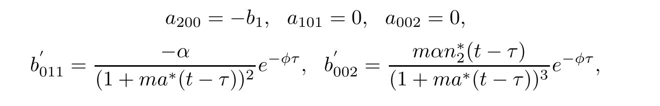
the coefficients of the linear terms are

and the coefficients of the nonlinear terms are as follows:

where u(t)=(u1(t),u2(t),u3(t))T∈ℜ3,Lµ:C→ℜ3,and f:ℜ×C→ℜ,for ϕ =(ϕ1,ϕ2,ϕ3)T∈ C([−1,0],ℜ3);

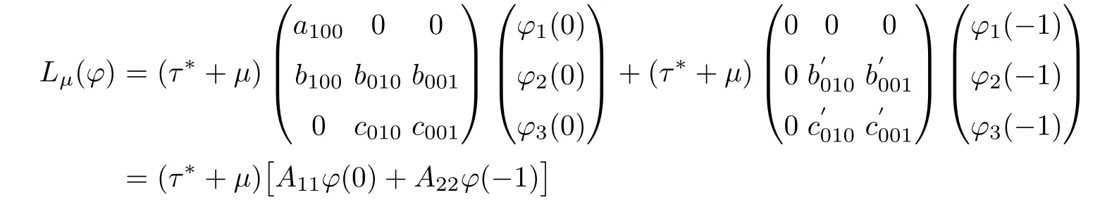
and

By Riesz representation theorem,there exists a 3×3 matrix function ς(θ,µ)of the bounded variation for θ∈ [−1,0],such that

In fact,we can choose

where δ denote the Dirac delta function.

For ϕ ∈ C([−1,0],ℜ3),we define

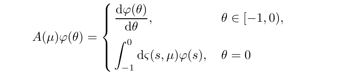
and

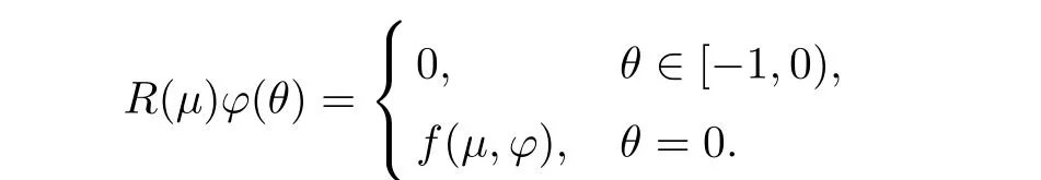
Then,system(7.2)is equivalent to

For ψ ∈ C1([0,1],(R3)∗),define

and a bilinear product

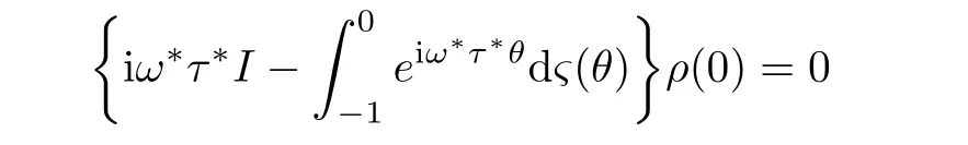
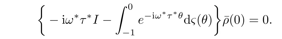
where ς= ς(θ,0).Then,A(0)and A∗are adjoint operators.From the results of last section,we know that ±iω∗τ∗are the eigenvalues of A(0),and they are also the eigenvalues of A∗.

Theorem 7.1Let ρ(θ)=(1,ρ1,ρ2)Teiω∗τ∗θ(θ∈ [−1,0))be the eigenvectors of A(0)corresponding to iω∗τ∗and

of A∗corresponding to −iω∗τ∗.

Then,〈ρ∗(s),ρ(θ)〉=1 and〈ρ∗(s),¯ρ(θ)〉=0,where

and

Next,we will compute the coordinates to describe the center manifold C0atµ=0.Let utbe the solution of(7.6)whenµ=0.

Define

On the center manifold C0,we have W(t,θ)=W(z(t),¯z(t),θ),where

or

where

From(7.8)and(7.9),we have

Now,from(7.3),it follows that

So,

where

As

we have

or

comparing coefficients of the above equation with(7.10),we find

As W20and W11are in g21,we are still to compute them.Now,from(7.6)and(7.8),we have

where

Substituting(7.14)into(7.13)and comparing the coefficients,we get

From(7.13)and for θ∈ [−1,0),

Using(7.10)in(7.16)and comparing the coefficients with(7.14),we get

and

From the definition of A(0),(7.15),and(7.17),we obtain

Solving it and for ρ(θ)=(1,ρ1,ρ2)Teiω∗τ∗θ,we have

Similarly,from(7.15)and(7.18),we obtain

Again from the definition of A(0)and(7.15),we have

and

where ς(θ)= ς(0,θ)

From(7.13),we know that when θ=0,

that is,

From(7.8),we have

From(7.3),we can also obtain

After substituting the value of f0(z,¯z)in(7.23)and comparing coefficients,we also have

As iω∗τ∗is the eigenvalue of A(0)corresponding to ρ(0)and −iω∗τ∗is the eigenvalue of A∗(0)corresponding to,then

and

Substituting(7.19)and(7.25)into(7.21),we find

which leads to

It follows that

where

Similarly,substituting(7.20)and(7.26)into(7.22),we have

where

Therefore,we can determine W20(θ)and W11(θ)from(7.19)and(7.20).Furthermore,g21can be computed from(7.12).Finally,we can compute the following quantities:

where gijis given by(7.12).The above quantities determine the qualities of bifurcating periodic solution in the center manifold at the critical value τ∗.By the above analysis,we state the following theorem.

Theorem 7.2The periodic solution is supercritical(subcritical)ifµ2＞ 0(µ2＜ 0);the bifurcating periodic solutions are orbitally asymptotically stable with asymptotical phase(unstable)if β2＜ 0(β2＞ 0);the period of the bifurcating periodic solutions increase(decrease)if T2＞0(T2＜0).

From the conclusions of Theorems 7.1 and 7.2,we can easily draw that the existence and stability of the bifurcation periodic solutions are only determined by the sign of Re(c1(0)).Specifically,if Re(c1(0))＜ 0,system(2.1)exists with stable periodic solutions for τ＞ τ∗in a τ∗-neighborhood.

8 Numerical Simulation

In this section,we shall carry out some numerical simulations for supporting our theoretical analysis.Our model involves various parameters,including the delay τ.In the following,we choose a set of parameters values and consider the following system:

The system has only a positive equilibrium point E∗(1.42,0.08805,0.0402),satisfies the local asymptotic stability condition H∗of E∗in the absence of time delay,and is shown in Figure 2.Numerically,by using the above said set of parametric values,for the delayed innovation diffusion system,a purely imaginary root iω∗from(5.2)with ω∗=0.8568 is calculated,and using it in(6.9),we have found the critical value of evaluation period τ= τ∗=2.1958 for the model system(8.1)such that E∗attains instability as τ passes through τ∗.Moreover,at τ= τ∗,the transversality conditionfor the existence of Hopf-bifurcation,is also satisfied,which proves that the interior equilibrium E∗remains locally asymptotically stable for 0≤ τ＜ 2.1958 and becomes unstable for τ≥ 2.1958(Figure 4).Figure 3 gives us stable dynamics of the innovation diffusion system for τ=1.9258.Also,an existence of Hopf-bifurcation in the form of a more stable limit cycle is shown for τ=2.2258 in Figure 5.Thus,it can be easily seen that there is a range of parameter′τ′such that the system attains local asymptotic stability around the positive equilibrium E∗for τ＜ τ∗and as τ crosses over this critical value of evaluation period,the system loses its stability and shows excitability in the form of limit cycle.This indicates that there is a threshold limit of evaluation period(τ,time taken by non adopter population to become the member of the adopter population class)below which the system produces local asymptotic stability and beyond this value,system shows excitable nature.

Also,we can calculate the stability determining quantities for the Hopf-bifurcating periodic solution at τ= τ∗as follows:

Therefore,using Theorem 7.2,it is apparent to know that the system has a stable center manifold near the positive equilibrium point E∗for τ near τ∗,the bifurcating periodic solutions are orbitally asymptotically stable on the center manifold,and the Hopf bifurcation is supercritical(see Figures 4,5).

The results obtained above shows that a smaller period required for innovation to be diffused in the market evaluation period has destabilizing effects on the innovation diffusion model system(8.1)by changing its states from locally asymptotically stable point to a limit cycle in the markets.

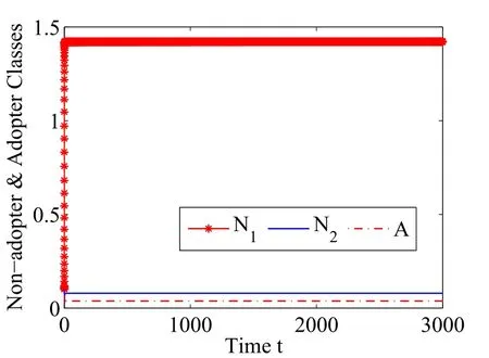
Figure 2 Solution trajectories predicting the local stability for Non-Adopter and Adopter Classes without any evaluation period τ

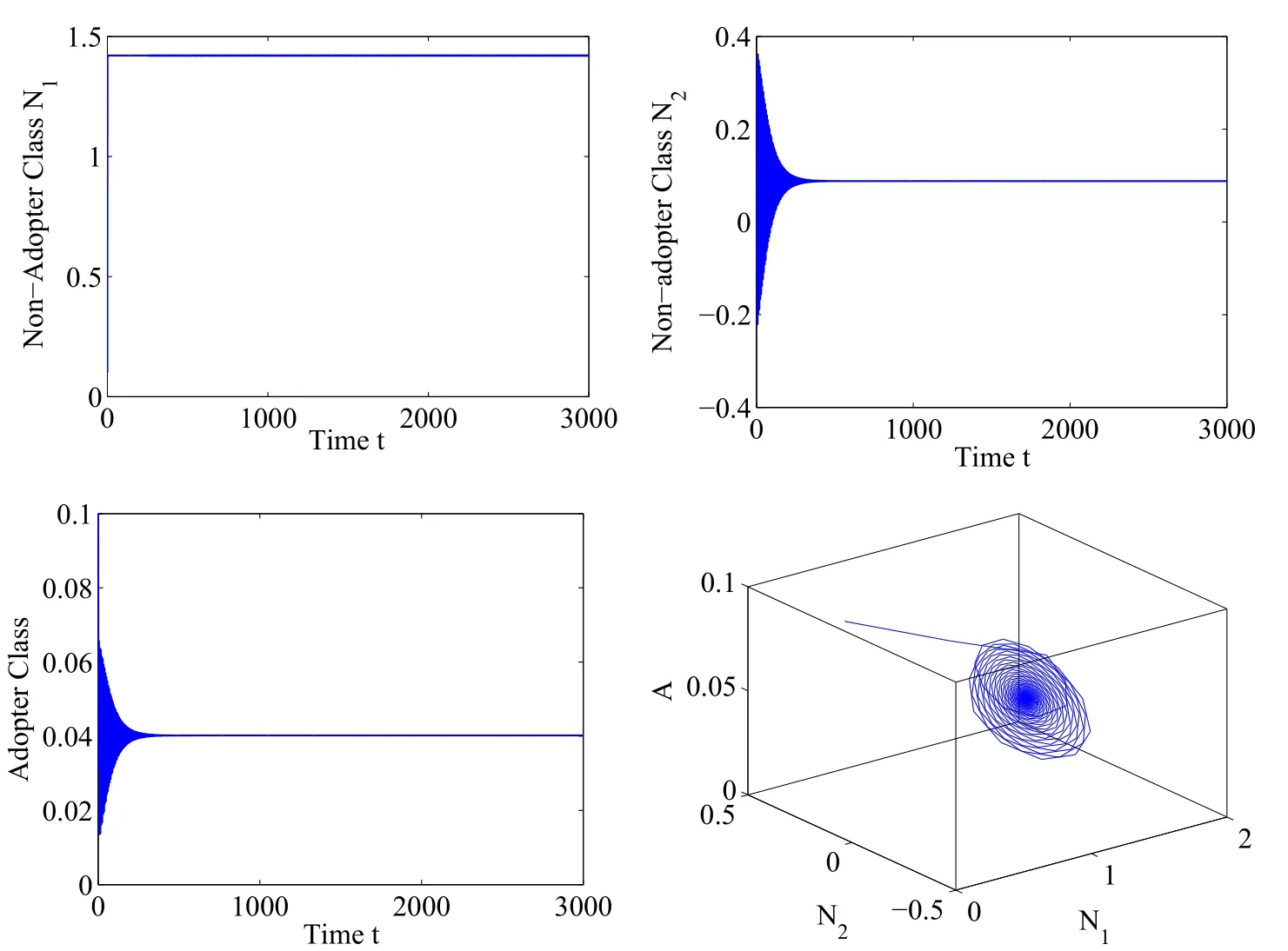
Figure 3 Convergence of solution trajectories to E∗(1.42,0.08805,0.0402)of system(2.2)at τ=1.9258＜τ∗with initial values(0.1,0.1,0.1)

Figure 4 Periodic oscillations of given system around E∗(1.42,0.1688,0.04667)for Non-Adopter and Adopter populations at τ=2.1958 with initial values(0.1,0.1,0.1)

Figure 5 Periodic oscillations of given system around E∗(1.42,0.1565,0.04587)for Non-Adopter and Adopter populations at τ=2.2258 with initial values(0.1,0.1,0.1)

9 Results and Discussion

In this article,the basic idea was to investigate the effect of evaluation period(time delay)on the innovation diffusion process of the system given by(2.1).Here,we observed that the system was producing local asymptotic stability without the evaluation period(Figure 2),that is,the given system does not have any excitable nature.But by the incorporation of evaluation period(τ),the stability of the system changes into Hopf bifurcation in the form of limit cycle,that is,there exist a certain threshold limit(0＜τ＜2.1958)beyond which the stability exchange take place and system shows periodic orbits around the positive equilibrium point E∗at τ=2.1958(Figure 4),which shows that as and when mature non-adopter population class(N2)does not think much before joining the adopter class(A),then both populations converges to some fixed values of the populations.Furthermore,when mature non-adopter population take sufficient time to think about the innovation before adoption,the innovation diffusion system becomes unstable and start producing periodic solutions.Moreover,using the normal form theory and center manifold theorem by Hassard et al[40],the direction and stability of bifurcating periodic solutions is determined by calculating the numerical values of c1(0),µ2,β2,and T2,and hence it is observed that the hopf bifurcation is supercritical in nature and the bifurcating periodic solutions are found to be asymptotically stable.Thus,we have found that evaluation period has a vital role to play in establishing the periodic orbits(that is,long term usage of new innovation by the members of the society)in the innovation diffusion model.Finally,the basic outcomes are mentioned along with numerical simulations to provide support to the analytical findings.Clearly,we have been able to show that some justifiable value of evaluation period is responsible for changing the stable innovation diffusion system to system with periodic cycles,that is,the adoption process starts and enter into the bifurcating periodic solutions.

[1]Fourt L A,Woodlock J W.Early prediction of market success for new grocery products.The Journal of Marketing,1960:31–38

[2]Mansfield E.Technical change and the rate of imitation.Econometrica:Journal of the Econometric Society,1961:741–766

[3]Bass F.A new product growth model for consumer durables.Management Science,1969,15:215–227

[4]Hale J K.Ordinary Differential Equations.New York:Wiley,1969

[5]Sharif M N,Kabir C.A generalized model for forecasting technological substitution.Technological Forecasting and Social Change,1976,8(4):353–364

[6]Sharif M N,Ramanathan K.Binomial innovation diffusion models with dynamic potential adopter population.Technological Forecasting and Social Change,1981,20(1):63–87

[7]Easingwood C,Mahajan V,Muller E.A nonsymmetric responding logistic model for forecasting technological substitution.Technological forecasting and Social change,1981,20(3):199–213

[8]Mahajan V,Muller E,Kerin R A.Introduction strategy for new products with positive and negative word-of-mouth.Management Science,1984,30(12):1389–1404

[9]Skiadas C.Two generalized rational models for forecasting innovation diffusion.Vol 27.Elsevier,1985

[10]Skiadas C H.Innovation diffusion models expressing asymmetry and/or positively or negatively in fluencing forces.Technological Forecasting and Social Change,1986,30(4):313–330

[11]Mahajan V,Peterson R A.Models for innovation diffusion.Vol 48.Sage,1985

[12]Dockner E,Jorgensen S.Optimal advertising policies for diffusion models of new product innovation in monopolistic situations.Management Science,1988,34(1):119–130

[13]Mahajan V,Muller E,Bass F M.New product diffusion models in marketing:A review and directions for research//Diffusion of technologies and social behavior.Springer,1991:125–177

[14]Rogers E M.Diffusion of innovations.New York:The Free Press,1995

[15]Horsky D,Simon L S.Advertising and the diffusion of new products.Marketing Science,1983,2(1):1–17[16]Mahajan V,Muller E,Bass F M.New-product diffusion models.Handbooks in Operations Research and Management Science,1993,5:349–408

[17]Dhar J,Tyagi M,Sinha P.Dynamical behavior in an innovation diffusion marketing model with thinker class of population.International Journal of Business Management Economics and Research,2010,1:79–84[18]Dhar J,Tyagi M,Sinha P.The impact of media on a new product innovation diffusion:A mathematical model.Boletim da Sociedade Paranaense de Matemática,2014,33(1):169–180

[19]Kuang Y.Delay differential equations:with applications in population dynamics.New York:Academic Press,1993

[20]Fergola P,Tenneriello C,Ma Z,Petrillo F.Delayed Innovation Diffusion Processes with Positive and Negative Word-of-Mouth.International Journal Differential Equations Application,2000,1:131–147

[21]Kot M.Elements of mathematical ecology.Cambridge University Press,2001

[22]Wang W,Fergola P,Lombardo S,Mulone G.Mathematical models of innovation diffusion with stage structure.Applied Mathematical Modelling,2006,30(1):129–146

[23]Wendi W,Fergola P,Tenneriello C.Innovation diffusion model in patch environment.Applied Mathematics and Computation,2003,134(1):51–67

[24]Tenneriello C,Fergola P,Zhien M,Wendi W.Stability of competitive innovation diffusion model.Ricerche di Matematica,2002,51(2):185–200

[25]Yu Y,Wang W,Zhang Y.An innovation diffusion model for three competitive products.Computers&Mathematics with Applications,2003,46(10):1473–1481

[26]Yu Y,Wang W.Global stability of an innovation diffusion model for n products.Applied Mathematics Letters,2006,19(11):1198–1201

[27]Yu Y,Wang W.Stability of innovation diffusion model with nonlinear acceptance.Acta Mathematica Scientia,2007,27(3):645–655

[28]Centrone F,Goia A,Salinelli E.Demographic processes in a model of innovation diffusion with dynamic market.Technological Forecasting and Social Change,2007,74(3):247–266

[29]Shukla J,Kushwah H,Agrawal K,Shukla A.Modeling the effects of variable external in fluences and demographic processes on innovation diffusion.Nonlinear Analysis:Real World Applications,2012,13(1):186–196

[30]Hale J K.Functional differential equations.Berlin,Heidelberg:Springer,1971

[31]Luenberger D G D G.Introduction to dynamic systems;theory,models,and applications.1979

[32]Song Y,Wei J,Han M.Local and global hopf bifurcation in a delayed hematopoiesis model.International Journal of Bifurcation and Chaos,2004,14(11):3909–3919

[33]Li F,Li H.Hopf bifurcation of a predator–prey model with time delay and stage structure for the prey.Mathematical and Computer Modelling,2012,55(3):672–679

[34]Song Y,Yuan S.Bifurcation analysis in a predator–prey system with time delay.Nonlinear analysis:real world applications,2006,7(2):265–284

[35]Liu L,Li X,Zhuang K.Bifurcation analysis on a delayed sis epidemic model with stage structure.Electronic Journal of Differential Equations,2007,77:1–17

[36]Boonrangsiman S,Bunwong K,Moore E J.A bifurcation path to chaos in a time-delay fisheries predator–prey model with prey consumption by immature and mature predators.Mathematics and Computers in Simulation,2016,124:16–29

[37]Sharma A,Sharma A K,Agnihotri K.The dynamic of plankton–nutrient interaction with delay.Applied Mathematics and Computation,2014,231:503–515

[38]Segel L A,Edelstein-Keshet L.A primer on Mathematical models in biology.Siam,2013

[39]Kuznetsov Y A.Elements of Applied Bifurcation Theory.Third Edition.Applied Mathematical Sciences.Vol 112.New York:Springer Verlag,2004

[40]Hassard B D,KazarinoffN D,Wan Y H.Theory and applications of Hopf bifurcation.Vol 41.CUP Archive,1981

[41]Ruan S,Wei J.On the zeros of transcendental functions with applications to stability of delay differential equations with two delays.Dynamics of Continuous Discrete and Impulsive Systems Series A,2003,10:863–874

[42]Kar T,Pahari U.Modelling and analysis of a prey–predator system with stage-structure and harvesting.Nonlinear Analysis:Real World Applications,2007,8(2):601–609

[43]Faria T,Magalh˜aes L T.Normal forms for retarded functional differential equations with parameters and applications to hopf bifurcation.Journal of Differential Equations,1995,122(2):181–200

[44]Sharma A,Sharma A K,Agnihotri K.Analysis of a toxin producing phytoplankton–zooplankton interaction with Holling IV type scheme and time delay.Nonlinear Dynamics,2015,81(1/2):13–25

[45]Sharma A K,Sharma A,Agnihotri K.Bifurcation behaviors analysis of a plankton model with multiple delays.International Journal of Biomathematics,2016,9(6):1650086