Evaluating and Im proving wind Forecasts over South China:The Role of Orographic Parameterization in the GRAPES Model
2018-04-08ShuixinZHONGZitongCHENDaoshengXUandYanxiaZHANG
Shuixin ZHONG,Zitong CHEN,Daosheng XU,and Yanxia ZHANG
Guangdong Province Key Laboratory of Regional Numerical Weather Prediction,Institute of Tropical and Marine Meteorology,China Meteorological Administration,Guangzhou 510080,China
1. Introduction
The Global/Regional Assimilation and Prediction System for the Tropical Mesoscale Model(GRAPES TMM)has presented a high wind speed bias over South China(Zhong and Chen,2015).The wind bias causes deficiencies in model performance—for example,an underestimation of precipitation and an overestimation of temperature over South China(Zhong et al.,2016),and an overestimation of snow fall over East Asia(Choi and Hong,2015).Although the bias was alleviated by the inclusion of orographic drag parameterization(Zhong et al.,2016;Choi et al.,2017),it persists in the lower troposphere,in particular over complex terrain and in the planetary boundary layer(PBL).High wind bias is a widespread phenomenon over mountains and valleys(Cheng and Steenburgh,2005).Nevertheless,wind speed bias also exists in other mesoscale models[e.g.,the Weather Research and Forecasting(WRF)model(Skamarock et al.,2008;Lorente-Plazas et al.,2015)].
The orographic gravity wave drag(GWD)can exert forces by gravity wave dissipation,whereas the body forces on the flow can either accelerate or decelerate atmospheric winds(Kim et al.,2003).The wind bias thus may be caused by an unrealistic simulation of the drag generated by the subgrid-scale gravity wave(Lindzen,1981;Matsuno,1982;Miller et al.,1989).Thus,GWD parameterization is generally recognized as the critical component for most models(Kim and Arakawa,1995;M cLandress et al.,2012;Choi and Hong,2015).The topography adopted in GRAPES TMM is derived from horizontal interpolation by a four-point averaged scheme,which may cause the smoother topography used in the model.It probably leads to an underestimation of the total orographic drag and causes high wind speed bias,especially in the lower troposphere over South China.It is argued that unresolved topographic effects(UTEs)produce an additional drag to that generated by vegetation,which leads to an overestimation of the wind speed in WRF[Jime´nez and Dudhia,2012(JD12)].The influences of UTEs include small-scale orography(SSO)effects(e.g.,SSO drags derived by several hills inside a horizontal grid).This subgrid orographic drag was named turbulent orographic drag(Belcher and Wood,1996),and it may be of the same order of magnitude as the GWD(Sandu et al.,2016).Wood et al.(2001)represented the turbulent orographic drag using an explicit orographic stresspro file,which considers the effects of stability instead of the effective roughness length(ERL).Belcher and Wood(1996)argued that a low-order closure model produces larger orographic drag because it overestimates the shear stress,where drag is related to turbulence.
Several schemes of unresolved orography have been developed to alleviate wind speed bias(Georgelin et al.,2000;Beljaars et al.,2004;Rontu,2006;Sandu et al.,2016).Among them,three basic concepts are adopted in the parameterization of UTEs.The first is to use an ERL(Fiedler and Panofsky,1972),which enhances the grid cell vegetative roughness length;the second proposes the introduction of the sink term in momentum equations(Wood et al.,2001;Wilson,2002);and the third is based on the momentum sink term(MST)method,which multiplies friction velocity according to the terrain characteristics(Jim´enez and Dudhia,2012).These three schemes can improve the performance of numerical weather prediction(NWP)models,especially on surface wind simulations(Milton and Wilson,1996;Rontu,2006;Jim´enez and Dudhia,2013;G´omez-Navarro et al.,2015;Lee et al.,2015;Sandu et al.,2016).Parameterizations based on the MST method show certain advantages over those adopting the ERL method.The MST method shows no limitation of the lowest model level and takes orographic features into account(Beljaars et al.,2004;Jim´enez and Dudhia,2012).However,the smoother topography used in the model can potentially lead to an underestimation of the SSO drags.For instance,the height of the mountain used in the model is lower than reality,especially over small hills within a horizontal gird.It has been argued that wind speed overestimation at mountainous regions would be due to lack of representation of SSO drag in NWP models[e.g.,in the WRF model Jim´enez and Dudhia(2012)].
Another related characterization parameter of the surface wind in NWP models is friction velocity.It was found that excessive convection-induced turbulent m ixing under free convection can lead to an overestimation of friction velocity and impose excessive surface friction(Liu et al.,2004).The overestimation of friction velocity can thus reduce surface momentum and lead to excessively weak surface winds.Underprediction of daytime surface winds results from anunderestimation of downward momentum flux(Zhang and Zheng,2004)or overestimation of surface stress(Liu et al.,2004).Lorente-Plazas et al.(2016)enhanced the friction velocity by considering the turbulent orographic drag effect and stability effects,and the results demonstrated that the inclusion of stability effects improved simulated surface winds by alleviating the systematic daytime underestimation of the original scheme.
The present work aims to alleviate wind speed bias in the GRAPES TMM model.The SSO drag effects on surface winds are parameterized by considering the orographic features based on the JD12 scheme.The SSO drag effects are represented by adding a sink term in the momentum equations with the maximum height of the hills or mountains within the grid box.The modification could be important by compensating for the drag that is underestimated by the smoother terrain used in the static data.The modified scheme is implemented and coupled with the PBL parameterization scheme within the model physics package.The results are verified against wind observations over South China and reanalysis data.
2. Model con figuration and observations
2.1. Model description
The model used in this study is the new-generation Mesoscale Atmospheric Regional Model System(MARS)in operation over South China based on GRAPES TMM(Zhong et al.,2016).MARS focuses on short-range forecasting of mesoscale convective systems over South China.The resolution was updated to within 3 km in 2016,and it provides data four times daily(initialized at 0000,0600,1200 and 1800 UTC).The physics package used in this paper is the same as that used in Zhong and Chen(2015),but without the convective cumulus scheme.The simulation domain comprises 913×513 grid points,with a horizontal resolution of 3 km,as shown in Fig.1a.There are 60 layers in the vertical direction,and both the initial and lateral boundary fields are obtained from the 0.125°×0.125°forecast fields of the European Centre for Medium-Range Weather Forecasts(ECMWF),with the lateral boundary fields updated every 6 h.
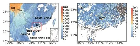
Fig.1. (a)Domain of MARS(3 km).Color shading denotes the orography,and the red frame shows the area of concern in(b).(b)The differences between h′and h;the dots denote the observation sites.
2.2. SSO parameterization
MARS uses a modified orographic parameterization scheme by including mountain blocking drag based on Kim and Arakawa(1995).This study focuses on the alleviation of wind bias through the implementation of the SSO parameterization(SSOP)scheme in MARS,based on the momentumcon servation equation(Jim´enez and Dudhia,2012).The topographic height(h)used in MARS is derived from horizontal interpolation by a four-point averaged scheme.In this paper,correction of the non-dimensional parameter of the topography Δ2hi,jis updated by using the maximum orography height(h′)from the U.S.Geological Survey at a horizontal resolution of 30 arc-seconds(Gesch et al.,2002).The differences betweenh′andhare shown in Fig.1b.It can be seen that the differences in subgrid orography can reach more than 200 m around Xinyi,west of Guangdong Province,South China.Thus,it employs the maximum heighth′of the mountains as compensation for drag being underestimated by the smoother terrainhused in the static data:
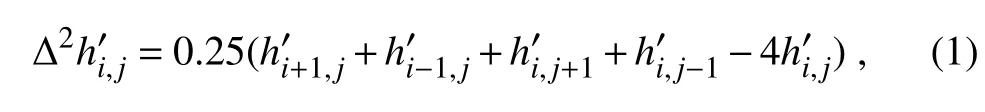
where positive values of Δ2hrepresent valleys and negative values indicate mountains;near-zero values indicate plains.The effects of the unresolved topography are parameterized,introducing a corresponding parameterctas a modulation of the surface drag associated with topography height in the calculation of the tridiagonal matrix elements(Hongetal.,2006)for momentum tendencies in PBL parameterization:
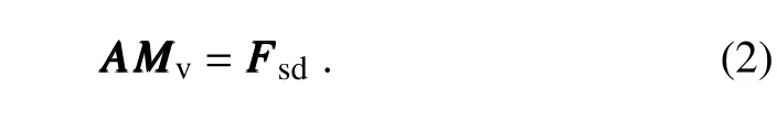
The vector of momentum tendencyMMMvis solved using the matrixAAAand forcingFFFsd,where the main diagonal ofAAAon the first model level is defined asA1:

Here,the subscript“1”stands for the first model level,ρ is the air density,gis the acceleration due to gravity,δ1represents the sink term,Sis the wind speed at the first model level,u∗is the friction velocity,and Δzis the thickness of the first model layer.ctis a function of Δ2and the standard deviation:where α′=Δ2h′+20/20 andeis the natural logarithm base.The standard deviationis also derived fromh′:
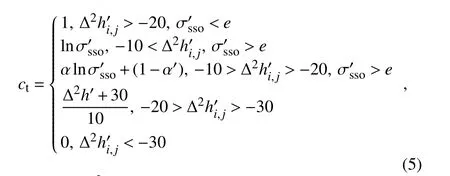

whereh′is the mean value in the grid box andNis the number of the grid box.A comprehensive description of the scheme and its numerical discretization is presented in the Appendix.
2.3. Topography and observations
The scheme is tested against wind observations over South China—a complex terrain region that includes the Nanling Mountains and Yunwu and Yunkai Mountains(YYMs),as well as the longest coastline in China(Fig.2a)and a complex underlying surface(mountains,plains,valleys,lakes,and so on).May 2016 is selected as the verification period;the main outbreak of the South Asian monsoon occurs during this period.The strong southerly winds bring abundant moisture and cause severe torrential rain,especially given the large-scale and small-scale mountains.Xinyi is characterized by a trumpet-shaped topography over the west of Guangdong Province(Fig.2b),where the north is dominated by the northern and western steep ridges of the YYMs and the south is covered by low valleys and areas of flat terrain.
式中:dIJ为目标回波的间隔距离;i,j=1,2,…,N;I=1,2,…,N;J=1,2,…,N。在目标回波中,若dIJ≤α,|H(Ai)-H(Aj)|
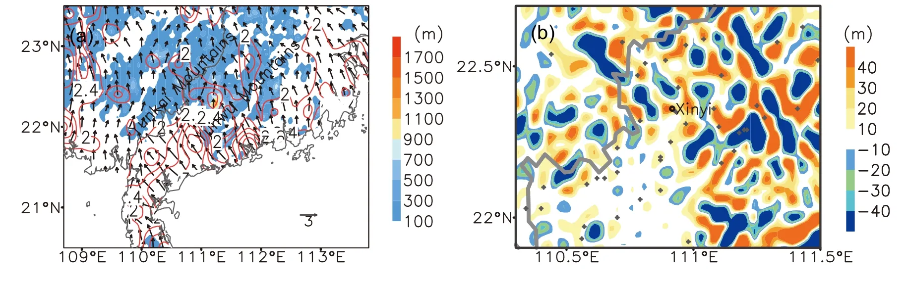
Fig.2. (a)The topography around Xinyi in the west of Guangdong Province and(b)the Δ2h′(negative values represent mountains,and positive values are valleys).The wind vectors(units:m s−1)in(a)are the five-day wind observation averages from 0800–1200 UTC,16–18 May 2016.The red contours in(a)denote surface wind speed(units:m s−1).
A total of 42 observational stations with conventional meteorological element measurements are used in the zoomed area in Fig.2,and around 8000 stations in the whole domain of MARS(Fig.1).These sites over the YYMs cover most of the region with a fine network.For instance,there are fifteen stations located over the flat region and five stations over the mountain region,as well as fourteen stations in the valleys and eight in the flat areas between mountains and valleys.The wind coverage shows that it is dominated by southeasterly wind over the flat areas in the south of Xinyi,with wind speeds of around 4 m s−1.Torrential rain occurred in association with the circulation over Xinyi on 20 May 2016.The 3D coverage of the topography,24-h rainfall and wind distribution are shown in Fig.3.It can be seen that precipitation was concentrated over the trumpet-shaped topography of Xinyi.The 24-h accumulated rainfall reached 464 mm,with southeasterly winds over the south and southeast of the Yunwu Mountains.
3. Results
3.1. Representativeness error analysis
The main diagonalAA Aat the first model level in Eq.(3)is related to the wind speed,friction velocity,thickness of the first model layer and topographic featuresct.For a given forcing term in Eq.(2),the wind speed becomes smaller asA1gets larger,and vice versa.Also,the value ofA1is proportional to the magnitude ofctand friction velocity.Figure 4 shows the distribution ofctandA1for the 50-timestep integration.It can be seen that the distribution ofctandA1shows good consistency with the topographic features in Fig.1.The distribution ofctin the steep mountainous region,especially over the Tibetan Plateau,is larger than those over the flat regions.Thus,the scheme could alleviate the wind speed in these mountainous regions as momentum tendency becomes smaller after considering subgrid orographic parameterization.
In addition,friction velocity is also an impact factor with respect toA1according to Eq.(4).Three experiments are set up in this study.Two of these experiments are the ORO and CTL experiments,which represent the SSOP scheme and control simulation,respectively.Figure 5 shows the feedback of the SSOP to the friction velocity in these two experiments.It can be seen that the friction velocity is alleviated after using the SSOP scheme in the ORO experiment.As enhanced friction velocity can lead to a largerA1in Eq.(4),and thus weaken the momentum tendency,this could lead to an underestimation of daytime winds(Liu et al.,2004).In this study,the results show that the friction velocity also becomes smaller,since the overestimated wind speed is alleviated(see section 3.2).However,the JD12 scheme may cause the underestimation of the daytime wind speed.Some other measures should be considered to alleviate this phenomenon;for instance,the effects of atmospheric stability could be included in the SSOP scheme(Lorente-Plazas et al.,2016),which is not discussed in this investigation.
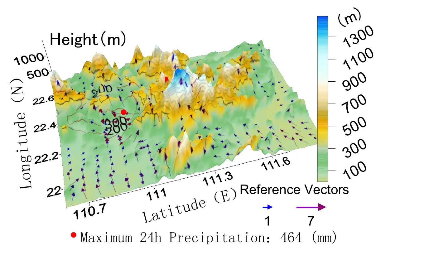
Fig.3. The 3D topographic features of Xinyi(color-shaded;units:m),24-h rainfall at 1200 UTC 20 May(contours;units:mm),and surface wind distribution at 0000 UTC 20 May 2016(vectors;units:m s−1).
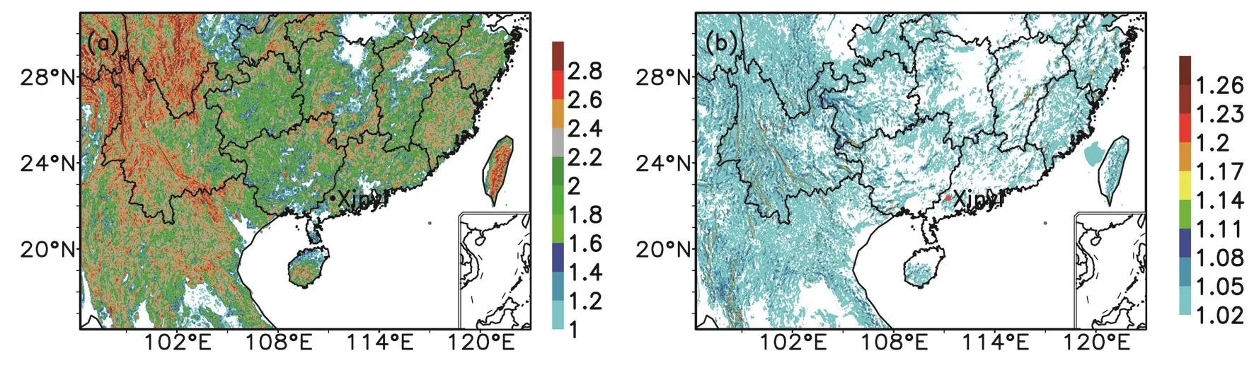
Fig.4. The distribution of(a)topographic function ct and(b)sink term A1 for the 50 time-step integration.
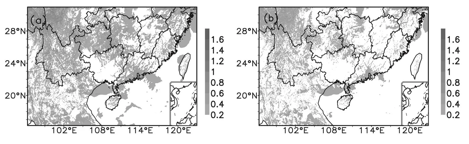
Fig.5. Comparison of the friction velocity(shaded;units:m s−1)of the 24-h simulation between(a)CTL and(b)ORO.
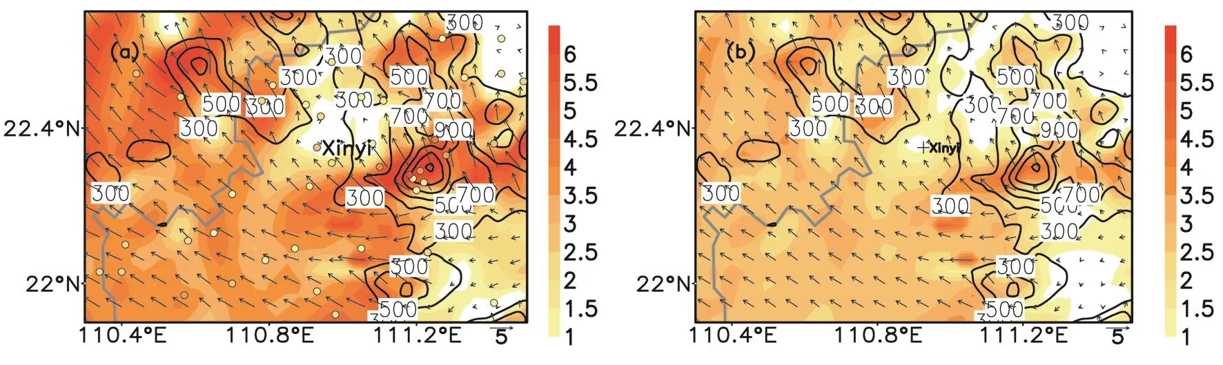
Fig.6. Comparison of the surface wind between the 12-h simulation(color-shaded)and the observation[colored dots(same color scale bar as the forecast);units:m s−1]at 0000 UTC 20 May,in which the contours represent the topography,for(a)CTL and(b)ORO.
3.2. Surface wind forecast performance
This study focuses on the subgrid orographic drag effects on low-level winds,especially the landing southerly winds from the South China Sea(e.g.,southwesterly winds brought by the monsoon),which have a strong influenc on the formation of the torrential rain over this complex terrain(Lin,2006).As mentioned,this investigation includes three experiments,including the ORO and CTL experiments introduced above,but also a third experiment of the JD12 scheme with the ORO experiment to examine the subgrid orographic effects.The Medium-Range Forecast(Hong et al.,2006)PBL scheme is used to verify the effects from the SSOP scheme,which is an independent code in the model physics process.
The surface winds of the ORO and CTL experiments are compared with observations in Fig.6.The two experiments share sim ilar simulated circulations,whereas the CTL experiment exhibits an obvious overestimation of wind speed.The magnitude of the wind speed over the flat regions reaches more than 3 m s−1in the CTL experiment,while the observations are around 1 m s−1.More overestimations are found over the mountains.For instance,the simulated winds reach more than 5 m s−1over the east and northwest of Xinyi,with observations around 3 m s−1.In contrast,the ORO experiment provides a much better simulated result than the CTL experiment,through a consistent magnitude with the observation over the flat regions and a slightly overestimated wind speed over the mountains.
The 850-hPa wind simulations are compared between the two experiments in Fig.7.A lthough both experiments share a similar simulation of the low-pressure vortex in the west of Xinyi,the southerly winds at the eastern edge of the vortex exhibit huge differences.The CTL experiment shows higher wind speeds than in the ORO experiment,with a smaller southerly wind zone over the eastern edge of the vortex.Another apparent difference in the two experiments is the southerly wind of the coastal regions over the southwest of Guangdong and the Beibu Gulf.The ORO experiment shows a larger southerly wind over the coastal areas,whereas the abundance of moisture accompanying the southerly wind may have a substantial influenc on the torrential rain over the terrestrial mountainous regions in the north.
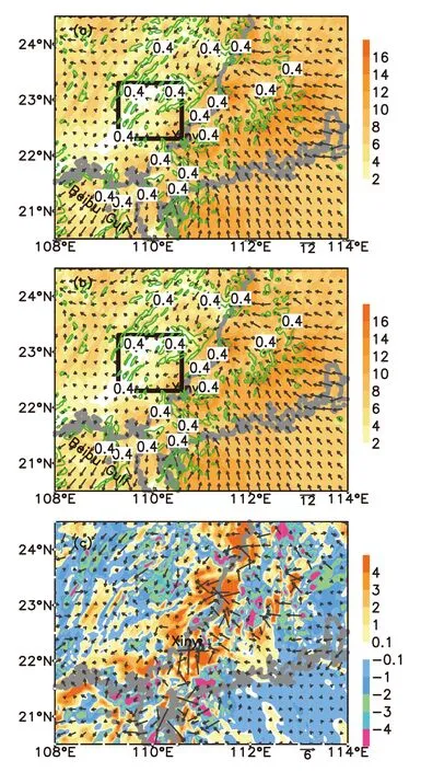
Fig.7. Comparison of the 850-hPa wind speed(color-shaded;units:m s−1)and relative vorticity(contours;>0.4×10⁻³ s−1)for the 24-h simulation at 1200 UTC 20 May between(a)CTL,(b)ORO and(c)ORO minus CTL,and the black frame shows the location of the vortex.
Figure 9a shows the vertical pro fi le of domain-averaged 24-h simulated wind speed.The two schemes have no significant influenc on the wind speed simulation,especially at layers higher than 800 hPa.Both schemes alleviate the wind speed between 1000 hPa and 800 hPa,and the 24-h wind speed simulation by the ORO scheme is slightly smaller than that of the JD12 scheme.The average wind pro files of the two experiments and the JD12 scheme over the coastal regions of southwestern Guangdong are compared in Fig.9b.The influenc of the scheme is more complicated,since it is related to the co-effects of the mountainous areas and coastal regions,and the feedbacks of the scheme to the wind speed can nearly reach 300 hPa,which is probably caused by the vertical transport of momentum and vertical diffusion in the PBL.Though both schemes can alleviate the wind speed,the ORO scheme provides a weaker wind speed than the JD12 scheme.Note,however,that revealing the sensitivity of the differences to the chosen scheme requires more experimentation,which is beyond the scope of this study.
3.3. Monthly verification
A monthly verification is executed to examine the stability and monthly performance of the SSOP scheme.This experiment is initialized twice daily at 0000 and 1200 UTC in May 2016,and the results are verified by the analysis field and observational station data,including the wind speed at 1000 hPa,925 hPa and 850 hPa by the analysis field,and the 10-m wind(V10m)and 2-m temperature(T2m)by the observations.Parameter verification is conducted by calculating the root-mean-square error(RMSE)between the forecast departure and real-case departure,the calculation of which is as follows:

whereSis the forecast value,Avis the analysis value(observation data),andNis the number of grid points in the verification region.The verification of wind speed at the isobaric level is employed in the ECMWF analysis field as the analysis value.The observations used in the verification of V10m and T2m are the observed ground-level surface synoptic observations(SYNOP)data collected by the South China Regional Meteorological Center at about 10 000 observation stations,some of which are shown in Fig.1b.
As can be seen from Table 1,the average 24-h and 48-h wind speed bias is greatly alleviated in the ORO experiment.For instance,the wind forecast error at 1000 hPa is alleviated from 4.67 m s−1to 2.18 m s−1,which is also verified using the V10m observations,with an error reduction of 2.99 m s−1and 3.1 m s−1from the 24-h and 48-h forecast(Table 2).Thereduction in 24-h wind speed RMSE at 925 and 850 hPa is 1.05 and 0.34 m s−1,respectively;plus,there are 48-h alleviations of 0.79 m s−1and 0.15 m s−1.The magnitude of the wind speed error reduction becomes weaker with a longer integration.On the other hand,the error reduction in the lower layer is more significant than that in the higher level,with a slight improvement in the T2m forecast(Table 2).The overestimated wind speed is thus reduced by including the SSO drags.
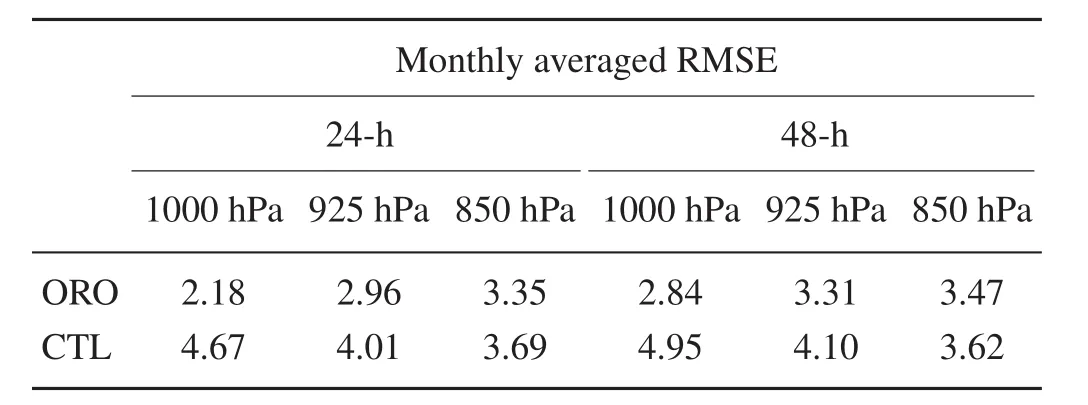
Table 1. Comparison of the monthly averaged RMSE of the 24-and 48-h forecasted wind speed(units:m s−1)at 1000,925 and 850 hPa.The verification is based on the RMSE between the forecast results and the corresponding analysis field from ECMWF.

Fig.8. As in Fig.7 but a comparison of the 850-hPa wind speed against the analysis(units:m s−1):(a)analysis minus CTL;(b)analysis minus ORO.
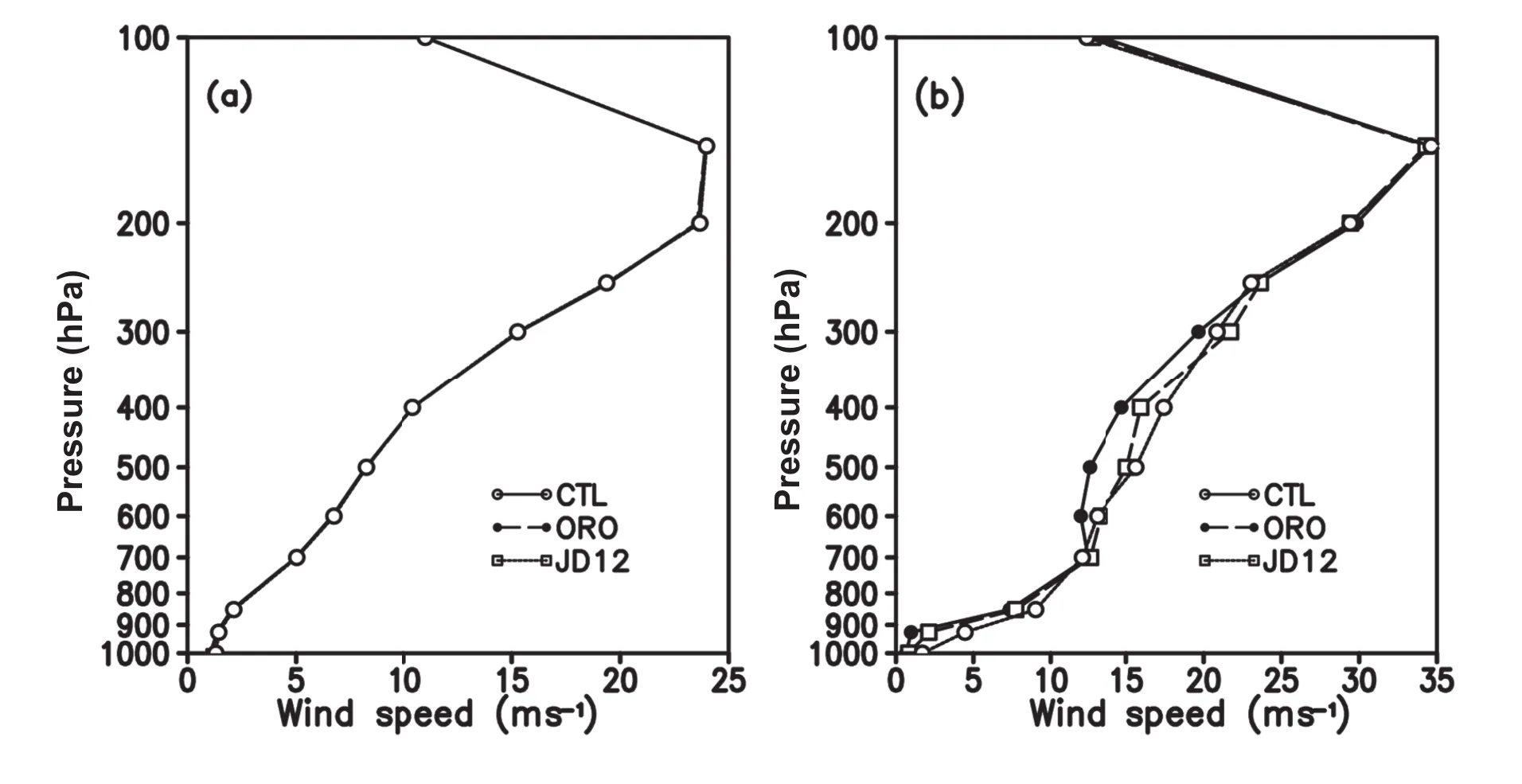
Fig.9. Comparison of the 24-h simulated wind pro file averaged(a)over the whole domain and(b)in the zoomed area in Fig.2.
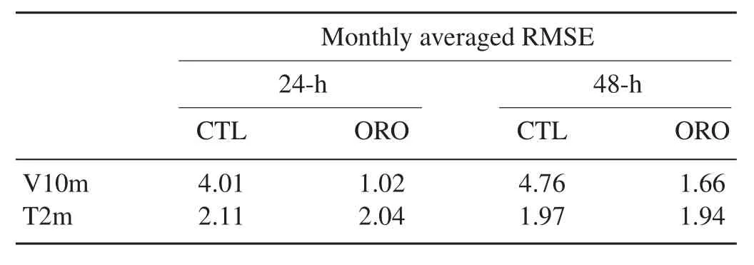
Table 2. Comparison of the monthly averaged RMSE of the 24-and 48-h for ecasted V10m(units:m s−1)and T2m(units:°C).The verification is based on the RMSE between the forecast results and site observations.
Figure 10 compares the monthly averaged surface wind between the 24-h simulation and the observations.It can be seen that the simulation without the SSOP scheme overestimates the surface wind over most of the region,especially over the flat regions in the south of Xinyi.The simulated winds over these regions reach more than 6 m s−1,while the observations are about 1–2 m s−1.Although both simulations can capture the strong wind speeds over the mountains,the simulation with the SSOP scheme provides a much better wind distribution over these regions,especially the flat regions over the south of Xinyi.Nevertheless,the simulated wind shows slight overestimation in some parts of the flat regions and underestimation over the Yunwu Mountains.
4. Discussion and conclusions

Fig.10. As in Fig.6 but a comparison of the monthly averaged surface wind between the 24-h simulation and the observations(units:m s−1):(a)CTL;(b)ORO.
Unresolved SSO drags are parameterized to improve the forecasting of surface winds in GRAPES TMM.The SSO drags are represented by adding a sink term in the momentum equations.A modification of the terrain features Δ2his calculated by the maximum height of the mountains within the grid box as a compensation for the drag.The scheme is implemented and coupled with the PBL parameterization scheme within the model physics package.A monthly simulation using the modified scheme outperforms the surface wind estimations and the default simulation over the complex terrain areas located in the southwest of Guangdong.
It is found that surface wind speed bias is greatly alleviated by adopting the SSOP scheme;this is also the case for surface temperature bias and wind bias in the lower troposphere,especially in the PBL.The monthly verification results show the wind forecast error at 1000 hPa to be alleviated from 4.67 m s−1to 2.18 m s−1,with an error reduction of 2.99 m s−1and 3.1 m s−1from the 24-h and 48-h forecast,respectively.The reduction in 24-h wind speed RMSE at 925 and 850 hPa is 1.05 and 0.34 m s−1,respectively;plus,48-h alleviations of 0.79 m s−1and 0.15 m s−1are also found.The veri fi cations between the simulation and observations show that,although both simulations can capture the strong wind speeds over the mountains,the simulation with the SSOP scheme provides a much better wind distribution over these regions,especially over the flat regions in the south of Xinyi.Nevertheless,the SSOP scheme still shows a slight overestimation over some parts of the flat regions and an underestimation over the Yunwu Mountains.
The results presented here show that the SSOP scheme in this paper to some extent outperforms the JD12 scheme.The SSO drags are strengthened by using a more realistic terrain height of the mountains,whereas the drags are underestimated with the current four-point averaging interpolation scheme in the static data.The SSOP scheme in this paper should be independent to the horizontal resolution used.Thus,more verifications should be designed with a more realistic terrain to evaluate SSO drags with different horizontal resolutions,and a more detailed verification of the performances with respect to the diurnal wind speed over other complex terrains should be exam ined.Moreover,the need to include stability effects should be considered to improve the diurnal characteristics of wind speed representation during the daytime and at nighttime.
Acknowledgements.Special thanks are given to the editors for the formula normalization.We also thank the reviewers for their helpful comments.This study was supported by the National Natural Science Foundation of China(Grant Nos.41505084,41275053 and 41461164006),the China Meteorological Administration Special Public Welfare Research Fund(Grant Nos.GYHY201406003 and GYHY201406009),the Guangdong Meteorological Service Project(Grant No.2015B01),and the Guang dong Province Public Welfare Research and Capacity Construction Project(Grant No.2017B020218003).
APPENDIX
The numerical formulation of the orographic parameterization scheme is discussed here.As is well known,the momentum equation may be written as
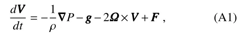
whereVVVis the horizontal wind,Pis the pressure,ρ is the atmospheric density, Ω is the angular velocity of the Earth andFFFis the turbulence forcing term,given by

whereDDDpblis the vertical diffusion term parameterized in the PBL,FFFgwdois the gravity wave drag induced by subgrid orography,FFFsdis the surface drag andFFFreis the rest of the frictional terms induced by subgrid processes,e.g.,the convective gravity wave drag(Bossuet et al.,1998;Song and Chun,2005)and turbulent drag(Lorente-Plazas et al.,2016).In JD12,the MST associated with surface drag in the momentum-conservation equation is
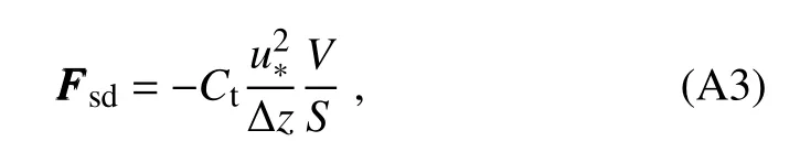
whereSis the wind speed at the first model level,u∗is the friction velocity,and Δzis the thickness of the first model layer.Ctis a function of the terrain characteristics.
The vertical diffusion for momentum equation in the PBL parameterization scheme of MARS is given by

whereKVis the momentum diffusivity coefficient,γvis a correction term of large-scale eddy motion for local gradients.The fi nite-difference centered-in-zform of Eq.(A4)is
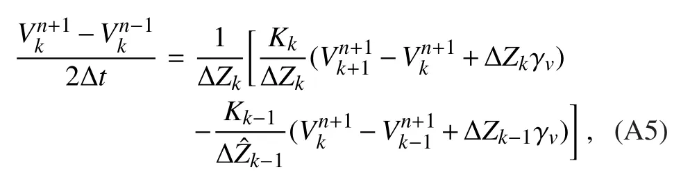
wherenis model integration time step,and we de fine:
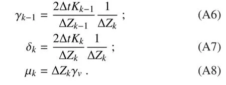
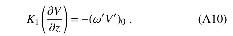
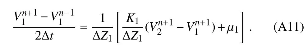
The general interior equation,for 1 For the top layer,k=Tx,the boundary condition isK(∂V/∂z)=0,and the lower boundary condition is The equation for the lowest layer,k=1,is now Recombination of the terms in Eqs.(A6),(A7)and(A11)yields: Equation(A13)can be simplified by The vector of momentum tendencyVVVis solved using the matrixAAAand forcingFFFfl,where the main diagonal ofAAAon the first model level is defined asA1. Belcher,S.,and N.Wood,1996:Form and wave drag due to stably strati fi ed turbulent fl ow over low ridges.Quart.J.Roy.Meteor.Soc.,122,863–902,https://doi.org/10.1002/qj.49712253205. Beljaars,A.C.M.,A.R.Brown,and N.Wood,2004:A new parametrization of turbulent orographic form drag.Quart.J.Roy.Meteor.Soc.,130,1327–1347,https://doi.org/10.1256/qj.03.73. Bossuet,C.,M.D´equ´e,and D.Cariolle,1998:Impact of a simple parameterization of convective gravity-wave drag in a stratosphere-troposphere general circulation model and its sensitivity to vertical resolution.Annales Geophysicae,16:238–249,https://doi.org/10.1007/s00585-998-0238-z. Cheng,W.Y.Y.,and W.J.Steenburgh,2005:Evaluation of surface sensible weather forecasts by the WRF and the Eta Models over the western United States.Wea.Forecasting,20,812–821,https://doi.org/10.1175/WAF885.1. Choi,H.J.,and S.Y.Hong,2015:An updated subgrid orographic parameterization for global atmospheric forecast models.J.Geophys.Res.,120,12 445–12 457,https://doi.org/10.1002/2015JD024230. Choi,H.J.,S.J.Choi,M.S.Koo,J.E.Kim,Y.C.Kwon,and S.Y.Hong,2017:Effects of parameterized orographic drag on weather forecasting and simulated climatology over East Asia during boreal summer.J.Geophys.Res.,122,10 669–10 678,https://doi.org/10.1002/2017JD026696. Fiedler,F.,and H.A.Panofsky,1972:The geostrophic drag coefficient and the‘effective’roughness length.Quart.J.Roy.Meteor.Soc.,98,213–220,https://doi.org/10.1002/qj.49709841519. Georgelin,M.,and Coauthors,2000:The second COMPARE exercise:A model intercomparison using a case of a typical mesoscale orographic fl ow,the PYREX IOP3.Quart.J.Roy.Meteor.Soc.,126,991–1029,https://doi.org/10.1002/qj.49712656410. Gesch,D.B.,M.J.Oimoen,S.K.Greenlee,C.A.Nelson,M.J.Steuck,and D.J.Tyler,2002:The national elevation data set.Photogrammetric Engineering and Remote Sensing,68(1),5–11. G´omez-Navarro,J.J.,C.C.Raible,and S.Dierer,2015:Sensitivity of the WRF model to PBL parameterisations and nesting techniques:Evaluation of wind storms over complex terrain.Geosci.Model Dev.,8,3349–3363,https://doi.org/10.5194/gmdd-8-5437-2015. Hong,S.Y.,Y.Noh and J.Dudhia,2006:A new vertical diffusion package with an explicit treatment of entrainment processes.Mon.Wea.Rev.,134,2318–2341,https://doi.org/10.1175/MWR3199.1. Jim´enez,P.A.,and J.Dudhia,2012:Improving the representation of resolved and unresolved topographic effects on surface wind in the WRF model.Journal of Applied Meteorology and Climatology,51,300–316,https://doi.org/10.1175/JAMC-D-11-084.1. Jim´enez,P.A.,and J.Dudhia,2013:On the ability of the WRF model to reproduce the surface wind direction over complex terrain.Journal of Applied Meteorology and Climatology,52,1610–1617,https://doi.org/10.1175/JAMC-D-12-0266.1. Kim,Y.J.,and A.Arakawa,1995:Improvement of orographic gravity wave parameterization using a mesoscale gravity wave model.J.Atmos.Sci.,52:1875–1902,https://doi.org/10.1175/1520-0469(1995)052<1875:IOOGWP>2.0.CO;2. Kim,Y.J.,S.D.Eckermann,and H.Y.Chun,2003:An overview of the past,present and future of gravity-wave drag parametrization for numerical climate and weather prediction models.Atmos.-Ocean,41,65–98,https://doi.org/10.3137/ao.410105. Lee,J.,H.H.Shin,S.Y.Hong,P.A.Jim´enez,J.Dudhia,and J.Hong,2015:Impacts of subgrid-scale orography parameterization on simulated surface layer wind and monsoonal precipitation in the high-resolution WRF model.J.Geophys.Res.,120,644–653,https://doi.org/10.1002/2014JD022747. Lin L.X.,2006:Technical Guidance on Weather Forecasting in Guangdong Province.China Meteorological Press,Beijing,236–244.(in Chinese) Lindzen,R.S.,1981:Turbulence and stress ow ing to gravity wave and tidal breakdown.J.Geophys.Res.,86,9707–9714,https://doi.org/10.1029/JC086iC10p09707. Liu,Y.B.,F.Chen,T.Warner,S.Werdlin,J.Bowers,and S.Halvorson,2004:Improvements to surface flux computations in a non-local-mixing PBL scheme,and re fi nements to urban processes in the NOAH land-surface model with the NCAR/ATEC real-time FDDA and forecast system.Proc.20th Conf.On Weather Analysis and Forecasting/16th Conf.on Numerical Weather Prediction,Seattle,WA,Amer.Meteor.Soc.,22.2.[Available online at https://ams.confex.com/ams/84Annual/techprogram/paper 72489.htm.] Lorente-Plazas,R.,J.P.Monta´vez,P.A.Jimenez,S.Jerez,J.J.Go´mez-Navarro,J.A.Garc´ıa-Valero,and P.Jimenez-Guerrero,2015:Characterization of surface winds over the Iberian Peninsula.International Journal of Climatology,35,1007–1026,https://doi.org/10.1002/joc.4034. Lorente-Plazas,R.,P.A.Jime´nez,J.Dudhia,and J.P.Monta´vez,2016:Evaluating and improving the impact of the atmospheric stability and orography on surface winds in the WRF model.Mon.Wea.Rev.,144,2085–2693,https://doi.org/10.1175/MWR-D-15-0449.1. Matsuno,T.,1982:A quasi one-dimensional model of the middle atmosphere circulation interacting with internal gravity waves.J.Meteor.Soc.Japan,60,215–226,https://doi.org/10.2151/jmsj1965.60.1 215. McLandress,C.,T.G.Shepherd,S.Polavarapu,and S.R.Beagley,2012:Is missing orographic gravity wave drag near 60°S the cause of the stratospheric zonal wind biases in chemistry–climate models?J.Atmos.Sci.,69,802–818,https://doi.org/10.1175/JAS-D-11-0159.1. Miller,M.J.,T.N.Palmer,and R.Sw inbank,1989:Parametrization and influenc of subgridscale orography in general circulation and numerical weather prediction models.Meteor.Atmos.Phys.,40,84–109,https://doi.org/10.1007/BF01027469. Milton,S.F.,and C.A.Wilson,1996:The impact of parameterized subgrid-scale orographic forcing on systematic errors in a global NWP model.Mon.Wea.Rev.,124,2023–2045,https://doi.org/10.1175/1520-0493(1996)124<2023:TIOPSS>2.0.CO;2. Rontu,L.,2006:A study on parametrization of orography-related momentum fluxes in a synoptic-scale NWP model.Tellus A:Dynamic Meteorology and Oceanography,58,69–81,https://doi.org/10.1111/j.1600-0870.2006.00162.x. Sandu,I.,P.Bechtold,A.Beljaars,A.Bozzo,F.Pithan,T.G.Shepherd,and A.Zadra,2016:Impacts of parameterized orographic drag on the Northern Hem isphere winter circulation.Journal of Advances in Modeling Earth Systems,8,196–211,https://doi.org/10.1002/2015MS000564. Skamarock,W.C.,and Coauthors,2008:A description of the Advanced Research WRF version 3.NCAR Tech.Note NCAR/TN-4751-STR,113 pp.,https://doi.org/10.5065/D68S4MVH. Song,I.S.and H.Y.Chun,2005:Momentum flux spectrum of convectively forced internal gravity waves and its application to gravity wave drag parameterization.Part I:Theory.J.Atmos.Sci.,62,107–124,https://doi.org/10.1175/JAS-3363.1. Wilson,J.D.,2002:Representing drag on unresolved terrain as a distributed momentum sink.J.Atmos.Sci.,59,1629–1637,https://doi.org/10.1175/1520-0469(2002)059<1629:RDOUTA>2.0.CO;2. Wood,N.,A.R.Brown,and F.E.Hewer,2001:Parametrizing the effects of orography on the boundary layer:An alternative to effective roughness lengths.Quart.J.Roy.Meteor.Soc.,127,759–777,https://doi.org/10.1002/qj.49712757303. Zhang,D.L.,and W.Z.Zheng,2004:Diurnal cycles of surface winds and temperatures as simulated by five boundary layer parameterizations.Journal of Applied Meteorology,43,157–169,https://doi.org/10.1175/1520-0450(2004)043<0157:DCOSWA>2.0.CO;2. Zhong,S.X.,and Z.T.Chen,2015:Improved wind and precipitation forecasts over south China using a modified orographic drag parameterization scheme.Journal of Meteorological Research,29,132–143,https://doi.org/10.1007/s13351-014-4934-1. Zhong,S.X.,Z.T.Chen,G.Wang,W.G.Meng,and R.Huang,2016:Improved forecasting of cold air outbreaks over southern China through orographic gravity wave drag parameterization.Journal of Tropical Meteorology,22,522–534,https://doi.org/10.16555/j.1006-8775.2016.04.007.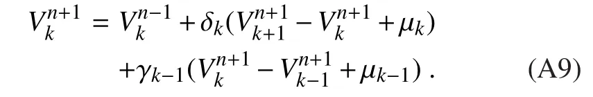


杂志排行

Advances in Atmospheric Sciences的其它文章
- Subseasonal Reversal of East Asian Surface Temperature Variability in winter 2014/15
- M odeling the warming Im pact of Urban Land Expansion on Hot Weather Using the Weather Research and Forecasting Model:A Case Study of Beijing,China
- Impact of the winter North Pacific Oscillation on the Surface Air Tem perature over Eurasia and North America:Sensitivity to the Index definition
- Regional Features and Seasonality of Land–Atmosphere Coup ling over Eastern China
- Simulating Eastern-and Central-Pacific Type ENSO Using a Sim p le Coup led M odel
- Evaluation of the New Dynamic Global Vegetation Model in CAS-ESM