Evaluation of the New Dynamic Global Vegetation Model in CAS-ESM

Jiawen ZHU,Xiaodong ZENG,M inghua ZHANG,Yongjiu DAI,Duoying JI,Fang LI,Qian ZHANG,He ZHANG,and Xiang SONG

1International Center for Climate and Environment Sciences,Institute of Atmospheric Physics,Chinese Academy of Sciences,Beijing 100029,China

2Collaborative Innovation Center on Forecast and Evaluation of Meteorological Disasters,

Nanjing University of Information Science and Technology,Nanjing 210044,China

3School of Marine and Atmospheric Sciences,Stony Brook University,NY 11790,USA

4School of Atmospheric Sciences,Sun Yat-Sen University,Guangzhou 510275,China

5College of Global Change and Earth System Science,Beijing Normal University,Beijing 100875,China

1.　Introduction

Land vegetation plays a pivotal role in regulating the exchange of heat,water,and carbon fluxes between the land surface and the atmosphere(Li and Xue,2010;Xue et al.,2010).The seasonal grow th of vegetation significantly impacts surface latent heat,downward and reflected solar radiation(Zhu and Zeng,2015,2017),and the interannual variability of vegetation can significantly regulate surface energy budgets via evapotranspiration(Guillevic et al.,2002;Zhu and Zeng,2016).Vegetation dynamics are considered to be as important for climate as atmospheric dynamics,ocean circulation(Pielke et al.,1998),and have gained much attention in recent years(Cramer et al.,2001;Seddon et al.,2016).

In the past several decades,rapid climate change has resulted in considerable changes in terrestrial ecosystems.One w idespread dynam ic change is the so-called“greening”of arctic ecosystems—a feature considered to be majorly contributed by boreal shrubs(Fraser et al.,2011;M yers-Sm ith et al.,2011).Both observation-and model-based studies have shown an increase in shrub biomass,coverage and abundance in arctic ecosystems in recent decades(Myers-Smith et al.,2011).Another key region is the tropics,which is ecologically sensitive to climate variability and shows ampli fi ed responses compared to other regions(Seddon et al.,2016).Many tropical ecosystems are more sensitive than other regions to environmentalperturbations and externaldisturbances,and are highly likely to cross a threshold to an alternative state(Holling,1973;Scheffer et al.,2009).

These vegetation changes can in turn significantly affect the climate.Over high latitudes,higher shrub abundance warms the winter soil temperature by trapping more snow via their branches(Sturm et al.,2001).During early spring,taller shrubs that expand into arctic tundra ecosystems also tend to systematically warm the soil because of their lower albedo than snow(Bonfils et al.,2012).In boreal summer,however,the shading imposed by shrubs is known to reduce the soil temperature and consequently the thickness of the active layer(Blok et al.,2010).Many studies have also reported that shrub canopies can alter arctic nutrient cycling,biodiversity and ecosystem services(Myers-Smith et al.,2011).Conversely,in the tropics,the complete deforestation of Amazonia may result in warmer,drier conditions at the local scale and lead to extratropical changes in temperature and rainfall through teleconnections(Lawrence and Vandecar,2015).Reduced plant cover in the Sahara,meanwhile,may cause a decline in precipitation because of the resultant increase in albedo(Charney et al.,1975),and the vegetation dynamics of West Africa have been shown to play a crucial role in regulating present-day climate,and probably future climate,via influenceson precipitation,evapotranspiration and energy balance(Erfanian et al.,2016;Yu et al.,2016).

Atpresent,Dynamic Global Vegetation Models(DGVMs)are the best available tool to represent vegetation dynamics at the global scale(Quillet et al.,2010).They can simulate transient and potential responses of vegetation to past and future climate change via parameterizing physical and biogeochemical processes of vegetation(Peng,2000).With the help of DGVM s,it is possible for global climate models(GCM s)to include the bidirectional interactions between vegetation and climate(Quillet et al.,2010).Therefore,the coupling of DGVMs and GCMs is an important approach to assess the influences of climate change on vegetation dynamics and their feedbacks to climate change.

However,there are still many uncertainties in reproducing and forecasting vegetation dynamics with DGVMs because of the complicated physical and biogeochemical processes.In response to climate change,most DGVMs simulate an increase in woody coverage over high latitudes,while others suggest a gain in herbaceous vegetation or no changes(Falloon et al.,2012).In terms of the Amazon ecosystem,the predictions from different models also vary widely,which is dominated by the differences in large-scale forest dieback and forest resilience(Betts et al.,2004;Friedlingstein et al.,2006;Baker et al.,2008;Restrepo-Coupe et al.,2017).Falloon et al.(2012)suggested that these responses of DGVM s to climate change are strongly associated with their simulation of present-day vegetation cover.Therefore,an important step to reduce these uncertainties in DGVMs is to systematically evaluate and understand their present-day performance,which is the main focus of the present study.

CoLM-DGVM is the default DGVM of the Common Land Model(CoLM).It was developed from the Lund–Potsdam–Jena DGVM(LPJ-DGVM;Sitch et al.,2003),and combined an early version of a temperate shrub sub-model of the DGVM developed at the Institute of Atmospheric Physics(IAP-DGVM;Zeng et al.,2008).In recent years,a boreal shrub sub-model,a process-based fire parameterization and a new establishment parameterization scheme have been further developed in IAP-DGVM.These developments have resulted in considerably improved reproductions of the presentday vegetation distribution and carbon cycle by IAP-DGVM(Zeng et al.,2014).At present,IAP-DGVM has been coupled to CoLM,and both are important components of the current version of the Chinese Academy of Sciences’Earth System Model(CAS-ESM).This work assesses the performance of IAP-DGVM,through comparison with that of CoLMDGVM,within the framework of CAS-ESM,which is a necessary step to using CAS-ESM for investigating vegetation–climate interactions.In the next section,the model,experimental design and observational data are described.The results are presented and discussed in section 3,followed by conclusions in section 4.

2.　M odel description,experimental design and observational data

2.1.　Model description

IAP-DGVM is a DGVM developed at the Institute of Atmospheric Physics,Chinese Academy of Sciences.It originates from LPJ-DGVM(Sitch et al.,2003)and the Community Land Model’s DGVM(CLM-DGVM;Levis et al.,2004).Plants in IAP-DGVM are classified into 14 plant functional types(PFTs)(Table 1),of which eight are trees,three are shrubs and three are grasses.These PFTs are defined by their physical,phylogenetic and phenological parameters,and are assigned bioclimatic limits to determine their establishment and survival.At present,crops are not simulated in IAP-DGVM.More details about the model can be found in Zeng et al.(2014).

In recent years,IAP-DGVM has undergone several major developments.These include the follow ing:(1)A shrub sub-model was established(Zeng et al.,2008;Zeng,2010).With this sub-model,IAP-DGVM can reproduce the global distribution of temperate and boreal shrubs realistically,and distinguish shrubs from grasses effectively(Zeng et al.,2008;Zeng,2010).(2)A process-based fire parameterization ofintermediate complexity was introduced(Li et al.,2012),which comprises fire occurrence, fire spread and fire impact.This fire parameterization significantly improves simulations of global fire,including burned area and fire carbon emissions(Li et al.,2013).The fire parameterization is now also adopted in the Community Earth System Model at the National Center for Atmospheric Research(NCAR)to investigate the influences of fire on carbon balance in terrestrial ecosystems,and on global land energy and water budgets(Li et al.,2014;Li et al.,2017;Li et al.,2017).(3)A new establishment parameterization scheme was developed(Song et al.,2016).This scheme significantly improves IAP-DGVM’s simulation of vegetation density by introducing soil water as an impact factor.These improvements,together with other optimized modifi cations,contribute to a better performance of IAP-DGVM in reproducing thepresent-day vegetation distribution and carbon cycle.

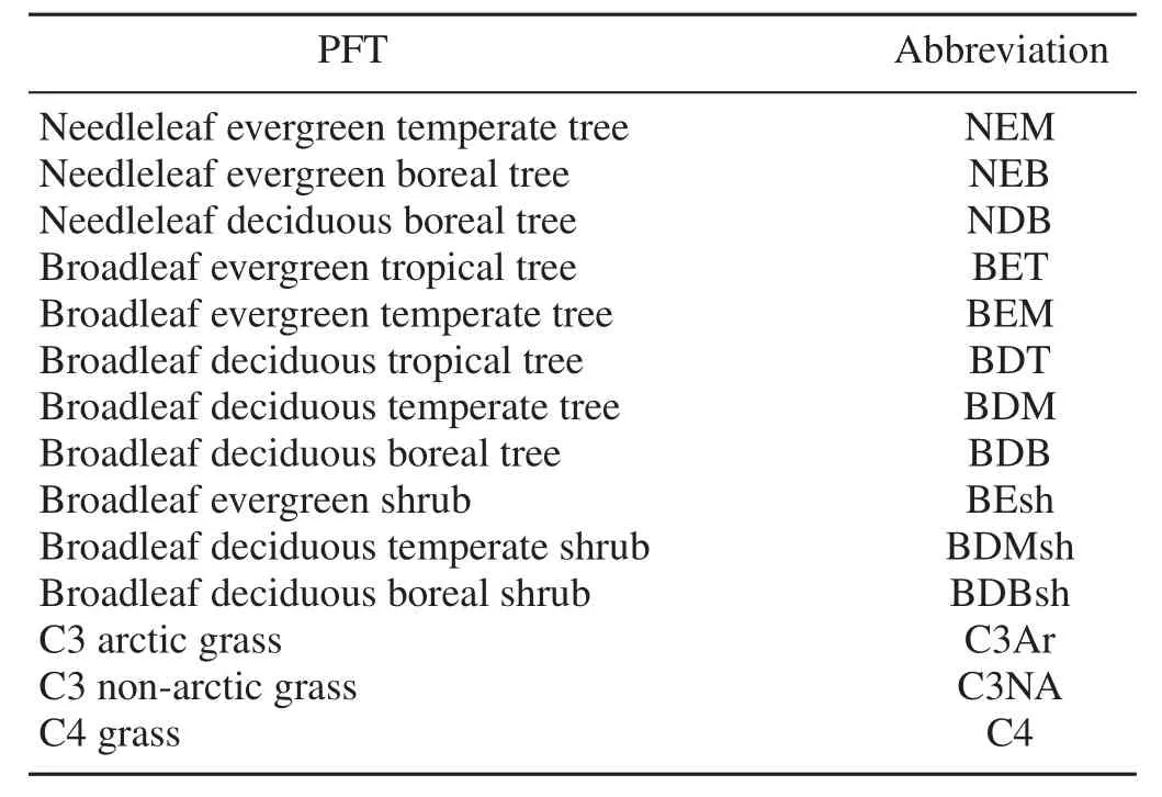
Table 1.　Plant functional types(PFTs)in IAP-DGVM and their corresponding abbreviations in this paper.

The land surface model used in this study is CoLM.Starting from the code of the NCAR’s Land Surface Model(Bonan,1996),Dai et al.(2003)developed the first version of CoLM,combining the codes of the Biosphere–Atmosphere Transfer Scheme(Dickinson et al.,1993)and the IAP’s land model(Dai and Zeng,1997).Since then,CoLM has been continually improved at Beijing Normal University in many aspects and has been adopted as the land component of the Beijing Normal University Earth System Model(Ji et al.,2014).

2.2.　Experimental design

Two global simulations were conducted within the framework of CAS-ESM.One,which coupled CoLM and CoLMDGVM,is the control(CTL)experiment,while the other,which coupled CoLM and IAP-DGVM,we refer to as IAP.Both simulations were spun up from bare ground for in excess of 1200 years.Then,a further 660 years were run to approach an equilibrium state through cycling the 33-year(1972–2004)atmospheric forcing data of Qian et al.(2006),with a T85 resolution(128×256 grid cells).The relative humidity and associated fire parameters needed for the IAP simulation were derived from Li et al.(2012)and fi xed in 2004.The atmospheric CO2was set to 365 ppmv over all simulated years.

2.3.　Observational data

This paper focuses on the vegetation distribution,carbon cycle and leaf area index(LAI).The observed vegetation distribution and LAI came from CLM 4 surface data,which were themselves derived from Moderate Resolution Imaging Spectroradiometer(MODIS)measurements(Law rence and Chase,2007).The benchmarks for gross primary productivity(GPP),net primary production(NPP)and fire carbon emissions were from Beer et al.(2010),MODIS(Zhao and Running,2010)and version 4 of the Global Fire emissions Database(GFEDv4;Randerson et al.,2015),respectively.The average of the last five years(2000–2004)of the IAP simulation was compared with that of CTL and these benchmarks.Furthermore,to reduce the impacts of crops,the vegetation cover in each grid cell was weighted by a factor of(100%-FCcrop),where FCcrop is the fraction of crop coverage in the CLM 4 surface dataset(Zeng et al.,2014).

3.　Results and discussion

3.1.　Vegetation distribution

Fig.1.　Zonal average fractional coverage(units:%)of(a)trees,(b)shrubs,(c)grasses and(d)bare groundin CTL(blue),IAP(red)and CLM 4 surface data(OBS;black).

In general,IAP simulated more realistic distributions for the four aggregated vegetation types(trees,shrubs,grasses and bare soil)than CTL.Over most latitudes,trees simulated by IAP were in better agreement with the observation,relative to CTL,which produced more trees(Fig.1a).In CTL,trees were overestimated over northern high latitudes,southeastern South America and A frica,with magnitudes of 50%(Fig.2a).Moreover,there was a band over central Eurasia where CTL’s trees were underestimated by more than 50%.In contrast,IAP simulated fewer trees over the tropics and more over central Eurasia than CTL,which resulted in a reduction in IAP’s biases(Fig.2b).Further investigation indicated that the new establishment scheme contributed most to the reduced biases of tropical trees,especially over transition zones(Song et al.,2016).

In terms of shrubs,both CTL and IAP underestimated them over arctic regions,such as northeastern Canada and the northern coastline of Eurasia(Figs.1b,2c and d).Further sensitivity experiments and analysis suggested that these underestimated shrubs were lim ited by the m inimum threshold of grow ing degree days over 5°C(GDD5)set by the model,which is 350.Shrubs were unable to establish because the annual GDD5 was smaller than 350.Over northern high latitudes,shrubs could not grow and were severely underestimated in the CTL simulation,while IAP simulated a more sim ilar shrub pattern than CTL with that observed(Fig.1b).This improvement can be attributed to the boreal shrub submodel of IAP-DGVM,which can distinguish shrubs from grasses effectively(Zeng et al.,2008;Zeng,2010).However,IAP simulated more shrubs than CTL over northern middle latitudes,such as western North America and central Eurasia,which further increases the biases of CAS-ESM.Moreover,both CTL and IAP underestimated the shrub coverage in the Southern Hem isphere,such as in Australia.

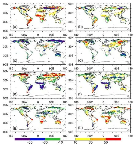
Fig.2.　Differences in fractional coverage(units:%)of(a)trees,(c)shrubs,(e)grasses and(g)bare ground between CTL and observations.(b,d,f,h)as in(a,c,e,g),respectively,but between IAP and observations.

IAP’s grasses also agreed better with the observation than those of CTL(Fig.1c).The grasses in CTL were largely overestimated over middle and high latitudes,such as northeastern Canada,central North America,middle and eastern Russia and central Eurasia,where the biases exceeded 50%.However,IAP reduced these deficiencies to around 10%over these regions(Fig.2f).Over the tropics,both CTL and IAP underestimated grasses,although IAP’s biases were a little smaller than those of CTL.The main underestimation was in southeastern South America and most regions of Africa.

Figure 1d shows that the bare soil simulated by CTL was underestimated over middle and high latitudes,and overestimated over the tropics,while IAP simulated more bare soil over almost all latitudes except southern middle latitudes.Over high latitudes,such as northeastern Canada,the underestimated bare soil of CTL mainly resulted from its overestimated grasses(Fig.2g).IAP significantly reduced the fractional coverage of grasses over northeastern Canada(Fig.2f);however,other vegetation,such as boreal shrubs,did not grow in this region(Fig.2d).Consequently,the bare soil of IAP was overestimated over northern high latitudes(Fig.2h).In the tropics,both CTL and IAP simulated more bare soil than observations(Fig.1d).These overestimations were mainly in northeastern Africa,southern Africa and Australia for CTL,and most regions of Africa for IAP(Fig.2h).The underestimated grasses were mostly responsible for these biases of tropical bare soil.

To investigate the contribution of each PFT to the improvements,Fig.3 shows the global average fractional coverage for each PFT in the two simulations and the observation.The total coverage of IAP’s trees(26.51%)was more consistent with that of the observation(28.51%)than that of CTL(35.60%).The smaller fractional tree coverage in IAP was mainly contributed to by a reduction in“broadleaf evergreen tropical tree”(BET;3.17%),“broadleaf deciduous tropical tree”(BDT;3.27%),“broadleaf deciduous temperate tree”(BDM;2.10%)and“broadleaf deciduous boreal tree”(BDB;2.10%).However,IAP’s BDT was less than half that of the observation,which was the major contributor to the underestimation of IAP’s total tree coverage.Further investigation indicated that the new establishment parameterization of IAP-DGVM resulted in this underestimated BDT,mainly over tropical semi-arid regions(Fig.S1 in electronic supplementary material).IAP also simulated 1.32%more“needleleaf evergreen boreal tree”(NEB)than CTL,which contributed to the band of increased tree coverage over central Eurasia apparent in Fig.2b.In terms of shrubs,the increased“broadleaf deciduous boreal shrub”(BDBsh)coverage(5.44%)in IAP was the main contributor to its better agreement with the observation than CTL.For grasses,although the total fraction in CTL was closer to that observed than IAP’s grass fraction,the“C3 arctic grass”(C3Ar)coverage in CTL was 6.33%larger than the observation,which corresponds to the severely overestimated grasses over high latitudes shown in Fig.1c.The composition of IAP’s grasses was generally in good agreement with the observation.However,the“C4 grass”(C4)coverage in IAP was 4.64%less than the observation,resulting in the underestimation of total grasses in IAP.The bare soil of CTL was close to that observed,but IAP simulated 7.67%more bare soil than the observation.The overestimated bare soil in IAP mainly resulted from its underestimated shrubs in arctic regions and underestimated grasses in the tropics(Fig.2).

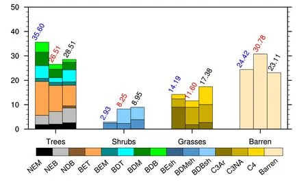
Fig.3.　Global weighted average fractional coverage(%)of each PFT for CTL(blue),IAP(red)and observation(black).The abbreviations correspond to the information in Table 1.

Fig.4.　Global distribution of the dominant vegetation type obtained from(a)CTL,(b)IAP and(c)observation.The abbreviations correspond to the information in Table 1.

Figure 4 shows the global distribution of the dominant vegetation type,which is the PFT with the highest fractional coverage.Clearly,the dominant vegetation simulated by IAP was more consistent with that obtained from the observation than that of CTL.In CTL,C3Ar dominated over most northern high-latitude regions.However,IAP showed the northern high latitudes to be dominated by bare soil,BDBsh and NEB,which was a sim ilar situation to that observed.In the tropics,CTL overestimated regions dominated by BET,as compared to observation.For example,BET was the dom inant vegetation in CTL over southeastern South America and West Africa,which,according to observation,are actually dominated by C4.With respect to CTL,IAP simulated fewer regions dominated by BET,which agreed well with observation.Nonetheless,IAP’s C4 was also not the dom inant vegetation in southeastern South America and West A frica because of the underestimated C4(Fig.3).

3.2.　Carbon fluxes

Compared to CTL,IAPsimulated an overallmore reasonable distribution of key carbon fluxes.Over most latitudes,the GPP in IAP was sim ilar to that of Beer et al.(2010),while CTL’s GPP was overestimated in middle and high latitudes(Fig.5a).The overestimated GPP in CTL stretched over the whole of central and eastern North America,Europe,South Asia and southeastern South America,while underestimated GPP dominated over the Amazon and Africa(Fig.6a).Relative to CTL,IAP’s GPP was closer to observation,especially over the Amazon(Fig.6b).Both CTL and IAP underestimated GPP over most regions of A frica.

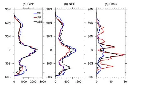
Fig.5.　Zonal average(a)GPP,(b)NPP and(c) fire carbon emissions(FireC)in CTL(blue),IAP(red)and the benchmarks(OBS;black).A ll units are gC m−2 yr−1.

In terms of NPP,IAP showed a better agreement with MODIS than CTL over northern high latitudes(Fig.5b).Relative to CTL,IAP simulated lower NPP over northeastern Canada and central and eastern Russia,where CTL simulated∼200 gC m−2yr−1more NPP than the observation(Fig.6c).Both CTL and IAP underestimated NPP over middle latitudes,mainly over arid and semi-arid regions.In the tropics,the simulated NPP in CTL was higher than the observation,mainly because of the overestimated NPP over the Amazon,West A frica and the Maritime Continent.On the contrary,IAP’s NPP was consistent with observations over the Amazon,Africa and the Maritime Continent.Both CTL and IAP underestimated the NPP over most parts of Africa.

Fire carbon emissions were overestimated by IAP over middle latitudes,especially in central and western North America,northeastern China,southern South America and Australia(Fig.6f).However,the fire carbon emissions simulated by IAP were much more consistent with observation in the tropics,where CTL showed a severe underestimation(Fig.5c).Fire carbon emissions in CTL were 10 gC m−2yr−1higher than the observation in eastern North America,Europe,the Amazon,Southeast Asia and the Maritime Continent,and 50 gC m−2yr−1lower in central South America and most regions of Africa(Fig.6e).IAP reduced these errors to different degrees by increasing or decreasing fire carbon emissions in these regions,respectively.Broadly,IAP captured a better spatial distribution of fire carbon emissions than CTL.

Overall,within the framework of CAS-ESM,IAP simulated carbon fluxes closer to observations than CTL,as summarized in Fig.7.The GPP simulated by IAP was 150.5 PgC yr−1,which is closer to the 123±8 PgC yr−1reported by Beer et al.(2010)than CTL’s GPP,and comparable to the range from 101 to 150 PgC yr−1published elsewhere(Farquhar et al.,1993;Ciais et al.,1997).Meanwhile,IAP also overestimated autotrophic respiration,which was almost the same as its counterpart in CTL.Consequently,IAP’s NPP,59.1 PgC yr−1,compared better with the expected value of 60 PgC yr−1(Castillo et al.,2012)than the result of CTL(75.31 PgC yr−1).Moreover,heterotrophic respiration in IAP was 56.20 PgC yr−1,which is closer to the 55.4 PgC yr−1from IPCC(2013)than that of CTL(74.08 PgC yr−1).Thus,the net ecosystem production in IAP was more reasonable than that in CTL,in comparison to the baseline from IPCC(2013).The fire carbon emissions in IAP were slightly higher than those of GFEDv4,because of the overestimated fire carbon emissions in the midlatitudes.Consequently,the net biome production(NBP)of IAP-DGVM was−0.2 PgC yr−1,which is outside the range of 2.63±1.22 PgC yr−1reported by other process-based terrestrial ecosystem models driven by rising CO2and by changes in climate(IPCC,2013).This nearzero value of NBP could be acceptable,however,because the results were based on the equilibrium state,which was cyclically forced by atmospheric datasets and a constant CO2value(Castillo et al.,2012).

3.3.　LAI

Generally,both CTL and IAP overestimated LAI,although the bias in IAP was smaller than that in CTL(Fig.8).The simulated annual mean LAI in CTL and IAP was 1.0 m2m−2more than the observation over most of the northern middle and high latitudes,such as central and eastern North America,Europe,central Eurasia and southeastern China.In the tropics,CTL’s bias in LAI exceeded 5.0 m2m−2,while IAP’s was∼3.0 m2m−2.In terms of seasonal variability,both CTL and IAP were consistent with observations,the largest being during June–August and the smallest during December–February.However,the simulated LAI ampli-tudes in CTL and IAP were around tw ice as large as those observed for each month.Although the LAI values in IAP were closer to observation compared to those of CTL,the improvements were not remarkable.Therefore,it is necessary to further investigate the causes of these systematically overestimated LAI values.

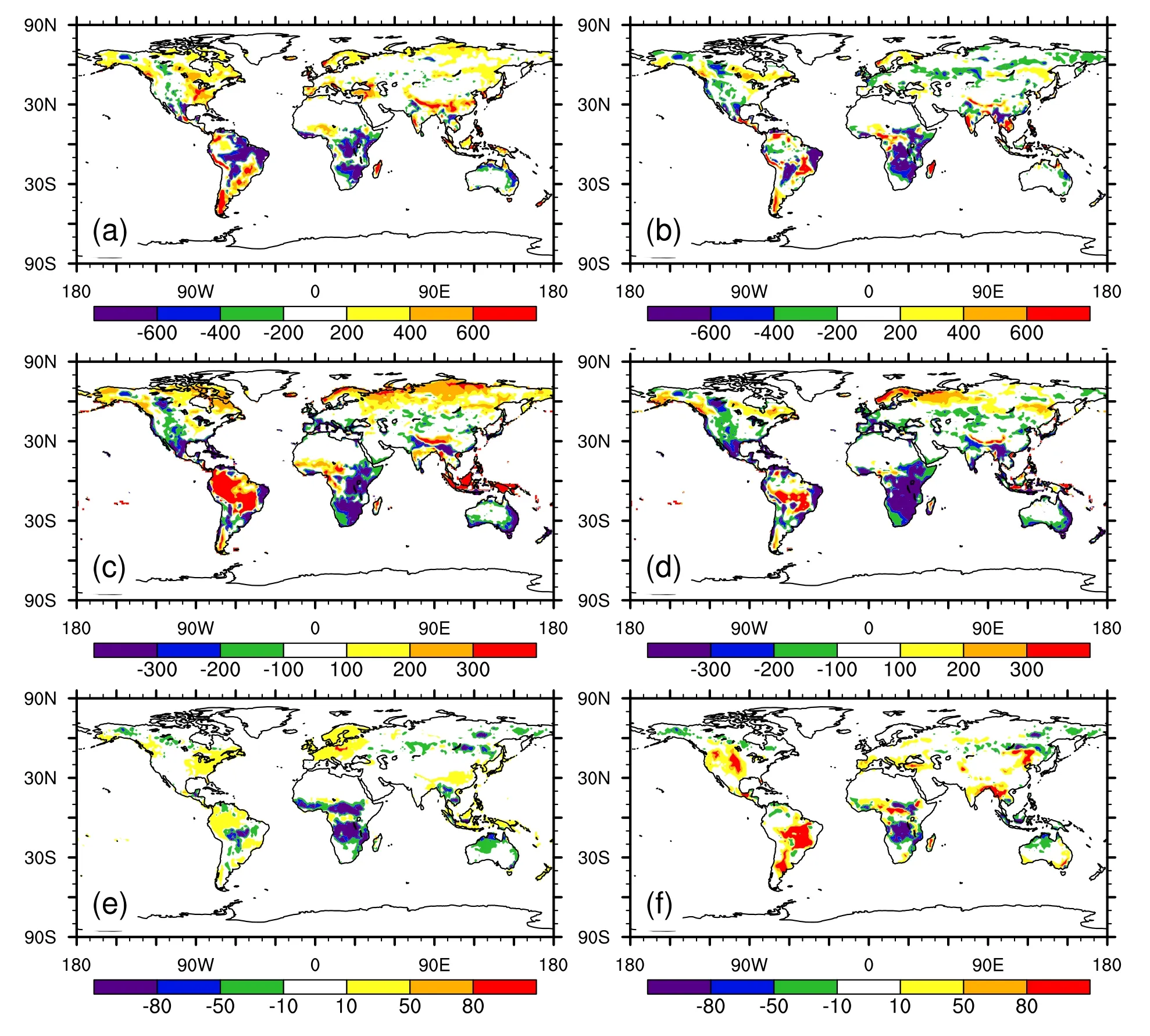
Fig.6.　Differences between CTL and the benchmarks(CTL minus benchmarks)in(a)GPP,(c)NPP and(e) fire carbon emissions(FireC).(b,d,f)As in(a,c,e),respectively,but between IAP and the benchmarks.All units are gC m−2 yr−1.

4.　Conclusions

This work evaluated the performance of IAP-DGVM within the framework of CAS-ESM through comparison with that of CoLM-DGVM,as well as observations and benchmarks.The results sufficiently demonstrated that IAPDGVM can simulate a realistic vegetation distribution,including spatial patterns,total areas and compositions,as well as reasonable carbon fluxes,such as GPP,NPP and fire carbon emissions.

The total tree coverage of IAP-DGVM was found to be in good agreement with observations,because of the reduced tropical trees and increased NEB relative to CoLM-DGVM.The shrub coverage in IAP-DGVM also showed a sim ilar distribution to that observed,which resulted from the significantly increased fractional coverage of BDBsh,with replacement of C3Ar.Meanwhile,the reduced C3Ar was the major contributor to the better consistency between the grass coverage in IAP-DGVM and that observed than between CoLMDGVM and that observed.Consequently,the global distribution of the dom inant vegetation type simulated by IAPDGVM was similar to that observed,especially over northern high latitudes.Moreover,the biases of IAP-DGVM in terms of GPP and NPP were smaller because of improvements in the GPP over middle and high latitudes,as well as in the tropics.The tropical patterns of fire carbon emissions in IAP-DGVM were much more consistent than CTL with observations.These better performances of IAP-DGVM in sim-ulating the global vegetation distribution and carbon fluxes provide a foundation to use CAS-ESM to study vegetation–climate interactions.

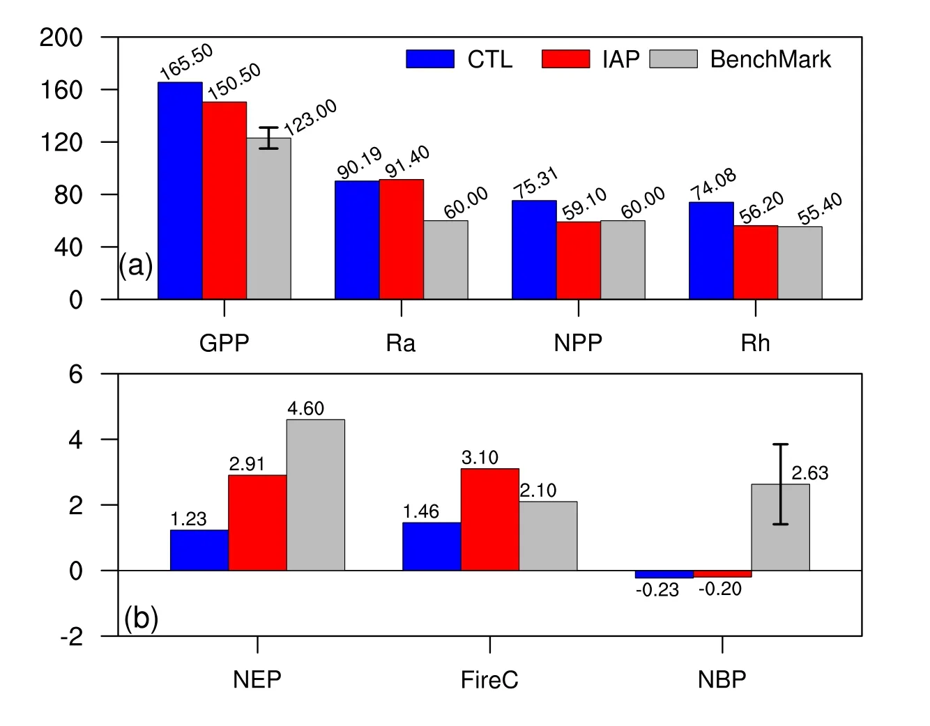
Fig.7.　Global means of carbon fluxes in CTL and IAP,as well as that of the benchmarks.Units:PgC yr−1.

Fig.8.　Differences in annual mean LAI between(a)CTL and observations,and(b)IAP and observations.(c)Globally averaged LAI in CTL(blue),IAP(red)and observations(black)for each month.A ll units are m2 m−2.

Despite the above positive results,deficiencies in IAPDGVM were also found.Speci fi cally,BDT was severely underestimated because of the new establishment parameterization;BDBsh could not grow in northeastern Canada because the simulated GDD5 did not exceed the threshold;and the C4 coverage was much smaller than the observation.Therefore,improved parameterization is necessary to simulate a more realistic distribution of vegetation types.Furthermore,both simulations overestimated GPP and autotrophic respiration,which is likely associated to the parameterization in CoLM being insufficiently sensitive to the DGVM.Additionally,the fire emissions simulated by the model in the high and middle latitudes were high.An understanding of the underlying mechanisms of these biases is needed to further improve the model,which will be the subject of future research.

The primary purpose of this study was to evaluate the performance of IAP-DGVM within the framework of CASESM,which makes the evaluations more model specific.However,this work also exerts the following influences on other studies.This study reported the improvements and deficiencies of IAP-DGVM in CAS-ESM,which is valuable information for the application of CAS-ESM,as well as a sample for other model communities in terms of a comparative benchmark.The selection of global observations of carbon fluxes in this study was limited by the spatial and temporal scale of existing datasets,which is a pivotal message for observational scientists to observe carbon fluxes with large spatial scale and continuous time.Overall,we hope that the advantages and disadvantages of the simulations reported in this paper will prove valuable for scientists seeking to investigate climate change.

Acknowledgements.This work was supported by the National Major Research High Performance Computing Program of China(Grant No.2016YFB02008)and the National Natural Science Foundation of China(Grant Number 41705070).Fang LI and Xiang SONG are supported by the National Natural Science Foundation of China(Grant Numbers 41475099 and 41305096).

Electronic supplementary material:Supplementary material is available in the online version of this article at https://doi.org/10.1007/s00376-017-7154-7.

Baker,I.T.,L.Prihodko,A.S.Denning,M.Goulden,S.Miller,and H.R.da Rocha,2008:Seasonal drought stress in the Amazon:Reconciling models and observations.J.Geophys.Res.,113,G00B01,https://doi.org/10.1029/2007JG000644.

Beer,C.,and Coauthors,2010:Terrestrial gross carbon dioxide uptake:Global distribution and covariation with climate.Science,329,834–838,https://doi.org/10.1126/science.1184984.

Betts,R.A.,P.M.Cox,M.Collins,P.P.Harris,C.Hunting ford,and C.D.Jones,2004:The role of ecosystem-atmosphere interactions in simulated Amazonian precipitation decrease and forest dieback under global climate warming.Theor.Appl.Climatol.,78,157–175,https://doi.org/10.1007/s00704-004-0050-y.

Blok,D.,M.M.P.D.Heijmans,G.Schaepman-Strub,A.V.Kononov,T.C.Maximov,and F.Berendse,2010:Shrub expansion may reduce summer permafrost thaw in Siberian tundra.Global Change Biology,16,1296–1305,https://doi.org/10.1111/j.1365-2486.2009.02110.x.

Bonan,G.B.,1996:A land surface model(LSM Version 1.0)for ecological,hydrological,and atmospheric studies:Technical description and user’s guide.NCAR Tech.Note NCAR/TN-417+STR,https://doi.org/10.5065/D6DF6P5X.

Bonfils,C.J.W.,T.J.Phillips,D.M.Lawrence,P.Cameron-Sm ith,W.J.Riley,and Z.M.Subin,2012:On the influenc of shrub height and expansion on northern high latitude climate.Environmental Research Letters,7,015503,https://doi.org/10.1088/1748-9326/7/1/015503.

Castillo,C.K.G.,S.Levis,and P.Thornton,2012:Evaluation of the new CNDV option of the community land model:Effects of dynamic vegetation and interactive nitrogen on CLM 4 means and variability.J.Climate,25,3702–3714,https://doi.org/10.1175/JCLI-D-11-00372.1.

Charney,J.,P.H.Stone,and W.J.Quirk,1975:Drought in the Sahara:A biogeophysical feedback mechanism.Science,187,434–435,https://doi.org/10.1126/science.187.4175.434.

Ciais,P.,and Coauthors,1997:A three-dimensional synthesis study of δ18O in atmospheric CO2:1.Surface fluxes.J.Geophys.Res.,102,5857–5872,https://doi.org/10.1029/96JD 02360.

Cramer,W.,and Coauthors,2001:Global response of terrestrial ecosystem structure and function to CO2and climate change:Results from six dynamic global vegetation models.Global Change Biology,7,357–373,https://doi.org/10.1046/j.1365-2486.2001.00383.x.

Dai,Y.J.,and Q.C.Zeng,1997:A land surface model(IAP94)for climate studies Part I:Formulation and validation in off-line experiments.Adv.Atmos.Sci.,14,433–460,https://doi.org/10.1007/s00376-997-0063-4.

Dai,Y.J.,and Coauthors,2003:The common land model.Bull.Amer.Meteorol.Soc.,84,1013–1023,https://doi.org/10.1175/BAMS-84-8-1013.

Dickinson,R.E.,A.Henderson-Sellers,and P.J.Kennedy,1993:Biosphere-Atmosphere Transfer Scheme(BATS)Version 1e as Coupled to the NCAR Community Climate Model.NCAR Tech.Note NCAR/TN-387+STR,72 pp,https://doi.org/10.5065/D67W 6959.

Erfanian,A.,G.L.Wang,M.Yu,and R.Anyah,2016:Multimodel ensemble simulations of present and future climates over West Africa:Impacts of vegetation dynamics.Journal of Advances in Modeling Earth Systems,8,1411–1431,https://doi.org/10.1002/2016MS000660.

Falloon,P.D.,R.Dankers,R.A.Betts,C.D.Jones,B.B.B.Booth,and F.H.Lambert,2012:Role of vegetation change in future climate under the A1B scenario and a climate stabilisation scenario,using the HadCM 3C Earth system model.Biogeosciences,9,4739–4756,https://doi.org/10.5194/bg-9-4739-2012.

Farquhar,G.D.,J.Lloyd,J.A.Taylor,L.B.Flanagan,J.P.Syvertsen,K.T.Hubick,S.C.Wong,and J.R.Ehleringer,1993:Vegetation effects on the isotope composition of oxygen in atmospheric CO2.Nature,363,439–443,https://doi.org/10.1038/363439a0.

Fraser,R.H.,I.Olthof,M.Carri`ere,A.Deschamps,and D.Pouliot,2011:Detecting long-term changes to vegetation in northern Canada using the Landsat satellite image archive.Environmental Research Letters,6,045502.

Friedlingstein,P.,and Coauthors,2006:Climate-carbon cycle feedback analysis:Results from the C4M IP model intercomparison.J.Climate,19,3337–3353,https://doi.org/10.1175/JCLI3800.1.

Guillevic,P.,R.D.Koster,M.J.Suarez,L.Bounoua,G.J.Col-latz,S.O.Los,and S.P.P.Mahanama,2002:influenc of the interannual variability of vegetation on the surface energy balance—A global sensitivity study.Journal of Hydrometeorology,3,617–629,https://doi.org/10.1175/1525-7541(2002)003<0617:IOTIVO>2.0.CO;2.

Holling,C.S.,1973:Resilience and stability of ecological systems.Annual Review of Ecology and Systematics,4,1–23,https://doi.org/10.1146/annurev.es.04.110173.000245.

IPCC,2013:Climate Change 2013:The Physical Science Basis.Contribution of Working Group I to the Fifth Assessment Report of the Intergovernmental Panel on Climate Change.T.F.Stockeretal.,Eds.,Cambridge University Press,1535 pp.

Ji,D.,and Coauthors,2014:Description and basic evaluation of Beijing Normal University Earth System Model(BNU-ESM)version 1.Geoscienti fi c Model Development,7,2039–2064,https://doi.org/10.5194/gmd-7-2039-2014.

Law rence,D.,and K.Vandecar,2015:Effects of tropical deforestation on climate and agriculture.Nat.Clim.Change,5,27–36,https://doi.org/10.1038/nclimate2430.

Law rence,P.J.,and T.N.Chase,2007:Representing a new MODIS consistent land surface in the Community Land Model(CLM 3.0).J.Geophys.Res.,112,G01023,https://doi.org/10.1029/2006JG000168.

Levis,S.,G.B.,Bonan,M.Vertenstein,and K.Oleson,2004:The Community Land Model’s dynam ic global vegetation model(CLM-DGVM):Technical description and user’s guide.NCAR Tech.Note TN-459+IA,50 pp,https://doi.org/10.5065/D6P26W 36.

Li,F.,and D.M.Law rence,2017:Role of fire in the global land water budget during the twentieth century due to changing ecosystems.J.Climate,30,1893–1908,https://doi.org/10.1175/JCLI-D-16-0460.1.

Li,F.,X.D.Zeng,and S.Levis,2012:A process-based fire parameterization of intermediate complexity in a Dynam ic Global Vegetation Model.Biogeosciences,9,2761–2780,https://doi.org/10.5194/bg-9-2761-2012.

Li,F.,S.Levis,and D.S.Ward,2013:Quantifying the role of fire in the Earth system—Part1:Improved global fire modeling in the Community Earth System Model(CESM 1).Biogeosciences,10,2293–2314,https://doi.org/10.5194/bg-10-2293-2013.

Li,F.,B.Bond-Lamberty,and S.Levis,2014:Quantifying the role of fire in the Earth system—Part 2:Impact on the net carbon balance of global terrestrial ecosystems for the 20th century.Biogeosciences,11,1345–1360,https://doi.org/10.5194/bg-11-1345-2014.

Li,F.,D.M.Law rence,and B.Bond-Lamberty,2017:Impact of fire on global land surface air temperature and energy budget for the 20th century due to changes within ecosystems.Environmental Research Letters,12,044014,https://doi.org/10.1088/1748-9326/aa6685.

Li,Q.,and Y.K.Xue,2010:Simulated impacts of land cover change on summer climate in the Tibetan Plateau.Environmental Research Letters,5,015102,https://doi.org/10.1088/1748-9326/5/1/015102.

Myers-Smith,I.H.,and Coauthors,2011:Shrub expansion in tundra ecosystems:dynamics,impacts and research priorities.Environmental Research Letters,6,045509,https://doi.org/10.1088/1748-9326/6/4/045509.

Peng,C.H.,2000:From static biogeographical model to dynam ic global vegetation model:A global perspective on modelling vegetation dynamics.Ecological Modelling,135(1),33–54,https://doi.org/10.1016/S0304-3800(00)00348-3.

Pielke,R.A.,R.Avissar,M.Raupach,A.J.Dolman,X.B.Zeng,and A.S.Denning,1998:Interactions between the atmosphere and terrestrial ecosystems:influenc on weather and climate.Global Change Biology,4,461–475,https://doi.org/10.1046/j.1365-2486.1998.t01-1-00176.x.

Qian,T.T.,A.G.Dai,K.E.Trenberth,and K.W.Oleson,2006:Simulation of global land surface conditions from 1948 to 2004.Part I:Forcing data and evaluations.Journal of Hydrometeorology,7,953–975,https://doi.org/10.1175/JHM 540.1.

Quillet,A.,C.H.Peng,and M.Garneau,2010:Toward dynamic global vegetation models for simulating vegetation-climate interactions and feedbacks:Recent developments,limitations,and future challenges.Environmental Reviews,18,333–353,https://doi.org/10.1139/A10-016.

Randerson,J.T.,G.R.Van Der Werf,L.Giglio,G.J.Collatz,and P.S.Kasibhatla.2015:Global Fire Emissions Database,Version 4,(GFEDv4).ORNL DAAC,Oak Ridge,Tennessee,USA,https://dx.doi.org/10.3334/ORNLDAAC/1293.

Restrepo-Coupe,N.,and Coauthors,2017:Do dynamic global vegetation models capture the seasonality of carbon fluxes in the Amazon basin?A data-model inter comparison.Global Change Biology,23,191–208,https://doi.org/10.1111/gcb.13442.

Scheffer,M.,and Coauthors,2009:Early-warning signals for critical transitions.Nature,461,53–59,https://doi.org/10.1038/nature08227.

Seddon,A.W.R.,M.Macias-Fauria,P.R.Long,D.Benz,and K.J.Willis,2016:Sensitivity of global terrestrial ecosystems to climate variability.Nature,531,229–232,https://doi.org/10.1038/nature16986.

Sitch,S.,and Coauthors,2003:Evaluation of ecosystem dynamics,plant geography and terrestrial carbon cycling in the LPJ dynamic global vegetation model.Global Change Biology,9,161–185,https://doi.org/10.1046/j.1365-2486.2003.00569.x.Song,X.,X.D.Zeng,J.W.Zhu,and P.Shao,2016:Development of an establishment scheme for a DGVM.Adv.Atmos.Sci.,33,829–840,https://doi.org/10.1007/s00376-016-5284-y.

Sturm,M.,J.Holmgren,J.P.McFadden,G.E.Liston,F.S.Chapin III,and C.H.Racine,2001:Snow-shrub interactions in Arctic tundra:A hypothesis with climatic implications.J.Climate,14,336–344,https://doi.org/10.1175/1520-0442(2001)014<0336:SSIIAT>2.0.CO;2.

Xue,Y.K.,F.De Sales,R.Vasic,C.R.Mechoso,A.Arakawa,and S.Prince,2010:Global and seasonal assessment of interactions between climate and vegetation biophysical processes:AGCM study with differentl and-vegetation representations.J.Climate,23,1411–1433,https://doi.org/10.1175/2009JCLI3054.1.

Yu,M.,G.L.Wang,and J.S.Pal,2016:Effects of vegetation feedback on future climate change over West A frica.Climate Dyn.,46,3669–3688,https://doi.org/10.1007/s00382-015-2795-7.

Zeng,X.D.,2010:Evaluating the dependence of vegetation on climate in an improved dynamic global vegetation model.Adv.Atmos.Sci.,27,977–991,https://doi.org/10.1007/s00376-009-9186-0.

Zeng,X.D.,F.Li,and X.Song,2014:Development of the IAP dynam ic global vegetation model.Adv.Atmos.Sci.,31,505–514,https://doi.org/10.1007/s00376-013-3155-3.

Zeng,X.D.,X.B.Zeng,and M.Barlage,2008:Grow ing tem-perate shrubs over arid and sem iarid regions in the Community Land Model-Dynam ic Global Vegetation Model.Global Biogeochemical Cycles,22,GB3003,https://doi.org/10.1029/2007GB003014.

Zhao,M.S.,and S.W.Running,2010:Drought-induced reductionin global terrestrial net primary production from 2000 through 2009.Science,329,940–943,https://doi.org/10.1126/science.1192666.

Zhu,J.W.,and X.D.Zeng,2015:Comprehensive study on the influence of evapotranspiration and albedo on surface temperature related to changes in the leaf area index.Adv.Atmos.Sci.,32(7),935–942,https://doi.org/10.1007/s00376-014-4045-z.

Zhu,J.W.,and X.D.Zeng,2016:influences of the interannual variability of vegetation LAI on surface temperature.Atmos.Oceanic Sci.Lett.,9(4),292–297,https://dx.doi.org/10.1080/16742834.2016.1189800.

Zhu,J.W.,and X.D.Zeng,2017:influences of the seasonal grow th of vegetation on surface energy budgets over middle to high latitudes.International Journal of Climatology,37,4251–4260,https://doi.org/10.1002/joc.5068.