Theoretical and numerical investigations of wave resonance between two floating bodies in close proximity ＊

Lei Tan (谭雷), Guo-qiang Tang (唐国强), Zhong-bing Zhou (周忠兵), Liang Cheng,2,3, Xiaobo Chen,Lin Lu(吕林),2

1. State Key Laboratory of Coastal and Offshore Engineering, Dalian University of Technology, Dalian 116023,China, E-mail: jerrytan@mail.dlut.edu.cn

2. DUT-UWA Joint Research Centre of Ocean Engineering, Dalian University of Technology, Dalian 116023,China

3. School of Civil, Environmental and Mining Engineering,The University of Western Australia,Crawley,Australia

4. Deepwater Technology Research Centre, Bureau Veritas, Singapore

Theoretical and numerical investigations of wave resonance between two floating bodies in close proximity＊

Lei Tan (谭雷)1, Guo-qiang Tang (唐国强)1, Zhong-bing Zhou (周忠兵)1, Liang Cheng1,2,3, Xiaobo Chen4,Lin Lu(吕林)1,2

1. State Key Laboratory of Coastal and Offshore Engineering, Dalian University of Technology, Dalian 116023,China, E-mail: jerrytan@mail.dlut.edu.cn

2. DUT-UWA Joint Research Centre of Ocean Engineering, Dalian University of Technology, Dalian 116023,China

3. School of Civil, Environmental and Mining Engineering,The University of Western Australia,Crawley,Australia

4. Deepwater Technology Research Centre, Bureau Veritas, Singapore

A simple theoretical dynamic model with a linearized damping coefficient is proposed for the gap resonance problem, as often referred to as the piston mode wave motion in a narrow gap formed by floating bodies. The relationship among the resonant response amplitude and frequency, the reflection and transmission coefficients, the gap width, and the damping coefficient is obtained.A quantitative link between the damping coefficient of the theoretical dynamic model ( ) and that devised for the modified potential flow model (up) is established, namely, up=3π εωn/8 (where ωnis the natural frequency). This link clarifies the physical meaning of the damping term introduced into the modified potential flow model. A new explicit approach to determine the damping coefficient for the modified potential model is proposed, without resorting to numerically tuning the damping coefficient by trial and error tests. The effects of the body breadth ratio on the characteristics of the gap resonance are numerically investigated by using both the modified potential flow model and the viscous RNG turbulent model. It is found that the body breadth ratio has a significant nonlinear influence on the resonant wave amplitude and the resonant frequency. With the modified potential flow model with the explicit damping coefficient, reasonable predictions are made in good agreement with the numerical solutions of the viscous fluid model.

Water wave, narrow gap, fluid resonance, energy dissipation, artificial damping

Introduction

The violent resonant oscillation of the water column in a narrow gap between two closely spaced floating structures may occur as the incident wave frequency is close to the natural frequency of the oscillating fluid mass. This phenomenon is often referred to as the gap resonance. The resonant wave in the narrow gap can bring about extreme local wave loads and large-amplitude motions of the floating structures, and hence affect the normal field operations, such as the side-by-side offloading/uploading operations between the liquefied natural gas (LNG)carriers and the Floating Liquefied Natural Gas(FLNG) platforms, and the ship berthing in front of a wharf.

In the past decades, the gap resonance problem has attracted much attention due to its engineering significance. The influence of the body draft and the gap width on the resonant characteristics was studied through physical experiments[1,2]. In addition, the previous investigations also include semi-analytical solutions and numerical simulations. Semi-analytical solutions[3-6]are mainly based on a potential flow assumption, and are limited to simple geometries.Numerical simulations involve two types of numerical models: the potential flow models and the viscous flow models. The potential flow models[7-11], based on the ass ump tion of irrotationa l flows of incompre ssible fluids,arecomputationallyefficient,however,theymight over-predict the resonant response amplitudes significantly due to the neglect of the energy dissipations.

Fig.1 (Color online) Sketch of gap resonance between two stationary floating bodies

Efforts have been made to modify the potential flow models by introducing a viscous damping mechanism (or a coefficient) while maintaining the computational efficiency. The modified potential flow models[12-16]can predict the resonant response accurately with a damping coefficient being tuned against experimental data. One of the uncertainties associated with the modified potential flow models is the way that the artificial damping coefficient is tuned through trial and error methods. Based on the experience in studying the liquid sloshing dynamics in a tank with a slatted screen, Faltinsen and Timokha[17]reported an empirical formula for estimating the damping coefficient instead of tuning it.

Viscous flow models were also proposed to investigate the fluid resonance in a narrow gap[18-23]in predicting successfully both the resonant frequency and the response amplitude. Moradi et al.[22]studied the effect of the energy dissipations on the resonant amplitudes through viscous model simulations of a gap resonance problem with various gap entrance corner configurations. It was found that the gap edge shape affects both the resonant frequency and the response amplitude. Although viscous fluid models can simulate the gap resonance problem accurately,they require huge computational resources.

However, the underlying physics behind the resonance characteristics in a gap remains unclear.The primary objective of the present work is to explore the relationship among the resonant response amplitude and frequency, the reflection and transmission waves, the body geometry and the damping for the gap resonance problem. Based on the physical understanding, a new approach is proposed to determine the artificial damping coefficient for the modified potential models. Furthermore, to the authors'knowledge, few of previous studies have considered the effects of the body breadth ratio on the resonant characteristics. In this work, both the viscous turbulent model and the modified potential flow model are used to examine the effect of the body breadth ratio.

This paper is organized as follows. After a brief introduction, a simple theoretical dynamic model with a linearized damping coefficient is proposed to describe the fluid resonance in a narrow gap. With the theoretical model, the artificial damping coefficient is quantified for the modified potential model. After that,a viscous turbulent model is used to simulate the gap resonance problem with different body breadths.Numerical results of the modified potential flow model are compared with the available experimental data and the present viscous numerical results. Finally,conclusions are drawn.

1. Fundamental theory

1.1 A theoretical dynamic model for gap resonance

A theoretical dynamic model for the motion of the oscillating fluid in the gap is proposed based on the concept of the control volume (CV). The gap resonance problem considered in this study is illustrated in Fig.1, where the wave-induced motions of the fluid trapped between two stationary bodies A and B are of the interest. A two-dimensional Cartesian coordinate system is defined with its origin located at the still water level and the middle section of the narrow gap, and the y-axis pointing vertically upwards.The incident wave propagates along x direction. The parameter his the water depth from the mean water level to the seabed,1B and2Bare the breadths of the bodies A and B, respectively,gBis the gap width and Dis the draft of the floating bodies A and B.

To analyze the wave induced motion of the fluid trapped in the gap, the energy conservation of the fluid enclosed by a CV is considered. The CV includes three regions, denoted by the regions 1, 2 and 3, as shown in Fig.1. The regions 2 and 3,corresponding to the area surrounded byoutside the gap that are influenced by the gap flow, as unknown a priori. The artificial parameter*B, which represents the summation of the breadths of the regions 2 and 3, can be determined through experimental calibrations or numerical calculations, which will be discussed in detail later on. The energy conservation equation over the CV reads

where t is the time, K and U are the total kinetic and potential energies contained in the CV,W is the rate of the work done on the CV andrepresents the rate of the energy flux across the boundary CS of the CV, where Q˙ is the power rate across the boundary CS. K and U can be, respectively, approximated as

where is the density of the fluid, Kj, Sjand Vjare the kinematic energy, the fluid volume and the mean flow velocity of the j - th region, respectively,gis the acceleration due to the gravity and η(t) is the amplitude of the fluid oscillation in the gap relative to the mean water level. The rate of the work done on the CV and the rate of the energy flux can be approximated as

where1F and2F are the forces acting on the surfaces12NN and N4N3, respectively, Wdrepresents the summation of the energy dissipation due to the friction forces on the CV surfaces (including the body surfaces and the seabed), the flow separations and the vortex shedding inside the CV. From the continuity conditions at the interfaces between the regions 1, 2 and 3, we have

By assuming V2≈V3, based on Eq.(6) and Eq.(2), and noting that V1=dη /dt, it is not difficult to obtain the total kinetic energy

Substituting Eqs.(3)-(5) and Eq.(7) into Eq.(1)and re-arranging, we have the motion equation of the fluid in the gap as

where

For the purpose of simplication, the nonlinear term in Eq.(8) is neglected. Thus Eq.(8) can be simplified as

Wdin Eq.(10) includes the contributions from the shear stress acting on the underside surfaces of the floating bodies and the seabed, the friction force acting on the side surfaces of the bodies in the narrow gap, and the energy dissipations in the CV. Based on the understanding of the flow head loss in hydraulics,Wdcan be written as

whereζ isa non-dimensional energy loss coefficient. As the fluid oscillation in the gap can be approximated by a harmonic response of η(t )= ηAcos(ω t-θ) with ηAbeing the response amplitude and the angular frequency, and the flow in the gap is in the vertical direction dominantly, we have

Substituting Eqs.(11)-(12) into Eq.(10), we have

The quadratic term in Eq.(13) can be further linearized[24], to finally lead to a linear motion equation

where F = Bg(F1+ F2)/[2(h - D ) /M ] represents the wave excitation force on the CV in total, ωnis the natural frequency of the water oscillation in the narrow gap

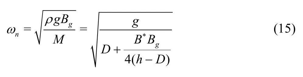
and is a non-dimensional damping coefficient of the oscillating system

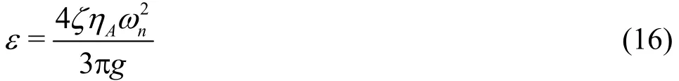
Equation(16)showsthat thesystem damping coefficient ε is dependent on the energy loss coefficient ζ, the response amplitudeAη and the natural frequencynω.

1.2 Energy dissipation

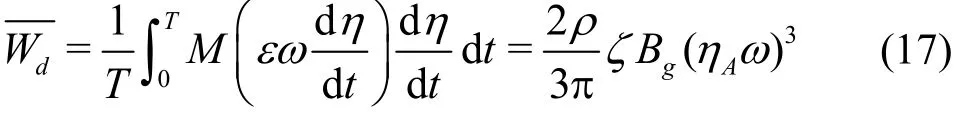
Based on Eq.(14), the average wave energy dissipation fluxover a wave period T is estimated as

On the other hand, based on the law of energy conservation, the incident wave energy fluxiP is equal to the summation of those due to the reflection waves, the transmission waves and the dissipative effects, which can be represented as

whererP ,tP anddP denote the reflected,transmitted and dissipated energy fluxes, respectively.Based on the linear wave theory, the three energy fluxes in Eq.(18) can be uniformly expressed as

where k is the wave number,,,irtA denote the wave amplitudes associated with the incident, reflection and transmission waves, respectively. By inserting Eq.(19)into Eq.(18), the dissipation ratedP can be expressed as

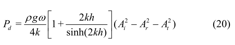
According to the definitions of the reflection coefficient and the transmission coefficient, namely,Kr= Ar/Aiand Kt= At/ Ai, the dissipative energy flux Pdcan be re-written as

where Kd=1-isa relativeenergy dissipation coefficient.

Indeed, Eq.(17) and Eq.(21) are two different approaches to estimate the energy dissipation in the gap resonance. Physically, the relationshipholds, which immediately leads to Substituting Eq.(16)intoEq.(22)and rearranging, we have

where the wave elevation response amplitude operator(RAO) is defined as. Equation (23) gives a quantitative relationship among the system damping coefficient ε (defined in Eq.(16)), the wave response amplitude RAOand the relative energy dissipation coefficient. Note that there are potential quantitative links between the system damping coefficient of the present theoretical model and the damping coefficients used by those modified potential models. Thus, with the aid of Eq.(23), it is possible to determine the damping coefficients of the modified potential models. This will be further discussed in the next section.

2. Numerical models

2.1 Modified potential flow model

In the framework of the conventional potential flow theory, the conservation of the mass is commonly expressed in the form of Laplace Equation in terms of the velocity potential

where Φ( x ,y,t ) is the velocity potential. Apart from Eq.(24), the potential Φ also satisfies the following boundary conditions:

where n is the outward normal unit vector.

In the modified potential models[12,15-16], in order to account for the damping induced by the vortex motion, the flow separations and the wall frictions, the dynamic boundary condition on the free surface in the gap is modified as

wherepμ is a dimensional damping coefficient. The above equation can be obtained by introducing a damping term into the momentum equation[12]. The introduced damping termdf reads

wheredf represents the damping force acting on the unit mass of the oscillating fluid. At the resonance, in a similar way as reported in Ref.[17], this damping force can be estimated by

where pΔ is the pressure drop which accounts for the viscous and friction damping induced by the fluid motion in the gap, M is the oscillating fluid mass in the gap resonance. Based on the understanding of the pressure loss in hydraulics, the pressure drop pΔ can be estimated by

Based on Eqs.(27)-(29), and Eq.(16) and noting that1=V▽, the relationship betweenpμ and ζ can be obtained, namely

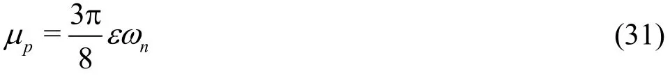
Note that the energy loss coefficient ζ in Eq.(30) is exactly the same as that in Eq.(11). Comparing Eq.(30)and Eq.(16), we can obtain the link between the damping coefficientpμ of the modified potential flow model and the damping coefficient of the theoretical dynamic model, i.e.,

By substituting Eq.(23) into Eq.(31), we can further obtain the following equation

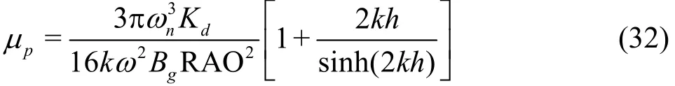
Equation (32) indicates that the damping coefficient pμ can be determined if the wave response amplitude RAO and the relative energy dissipation coefficientapproach to estimate the damping coefficient used in the modified potential models. The application of Eq.(32) will be shown later.

2.2 Viscous turbulent model

The governing equations of the incompressible

turbulent flows with the renormalization group (RNG)model can be written as follows:

where uiis the velocity component in the i-th direction, the pressure, the fluid density, fithe external body force, μethe effective dynamic viscosity with μe= μ + μt, the fluid viscosity and μtthe turbulent viscosity. Note that all flow variables in Eqs.(33)-(34) are filtered by the RNG procedure. In order to close the governing equations,the RNG k - two-equation formulationsare adopted, which gives

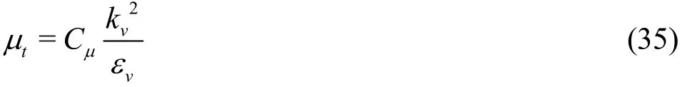
where Cμ=0.09 is a theoretical model constant, and the time-dependent advection-diffusion equations for the turbulent kinematic energy kvand its dissipation rate εvread

where the model constants of C1ε=1.42, C2ε=1.68,σk=0.71942 and σε=0.71942 are also derived theoretically, but not based on the experimental calibrations, as is distinct from the widely used Reynolds averaging Navier-Stokes (RANS) model.

The volume of fluid (VOF) metho is used to capture the free surface in the viscous fluid model. A fractional function of the VOF, denoted by φ in this paper, for a computational cell, is defined as:

The VOF function follows the advection equation

In this paper, the contour of the VOF function with =0.5φ is used to represent the interface between the water and air phases. In the computations,the fluid density and the effective viscosity are averaged by using the available VOF function

where the subscripts W and A represent the water phase and the air phase, respectively.

The numerical computations in this paper, always start from the still state, which allows the static water pressure and the zero velocity to be specified as the initial conditions. The no-slip boundary condition is imposed on the solid wall. At the upper boundary of the computational domain, the reference pressure p = 0 and the velocity condition ∂ u /∂ n =0 are implemented. The interface tension between the air and water phases is neglected. At the two ends of the wave absorption zones, zero velocities are imposed considering that the waves are damped out there. The momentum source method[26]is adopted to generate the incident linear waves. The necessary numerical verification and validation for the present viscous fluid model are presented in the Appendix of this paper.

3. Results and discussion

3.1 Viscous numerical solutions

The influence of the breadth ratio on the resonant response is first examined by using the viscous turbulent model. A sketch of the viscous numerical simulations of this paper is illustrated in Fig.2. Two fixed floating rectangular boxes, defined as Box A and Box B, respectively, are placed in a wave flume with a constant water depth h. A narrow gap with the width Bgis formed by the two boxes with an identical draft D. The breadths of the two boxes are denoted by B1and2B, respectively. Two numerical wave absorption zones are numerically arranged on the both ends of the wave flume in order to absorb the reflection waves. Four wave gauges G1-G4are used to record the wave elevations. In the numerical simulations, the breadth of the rear box2( )B is varied while the breadth of the leading box1( )B is fixed.

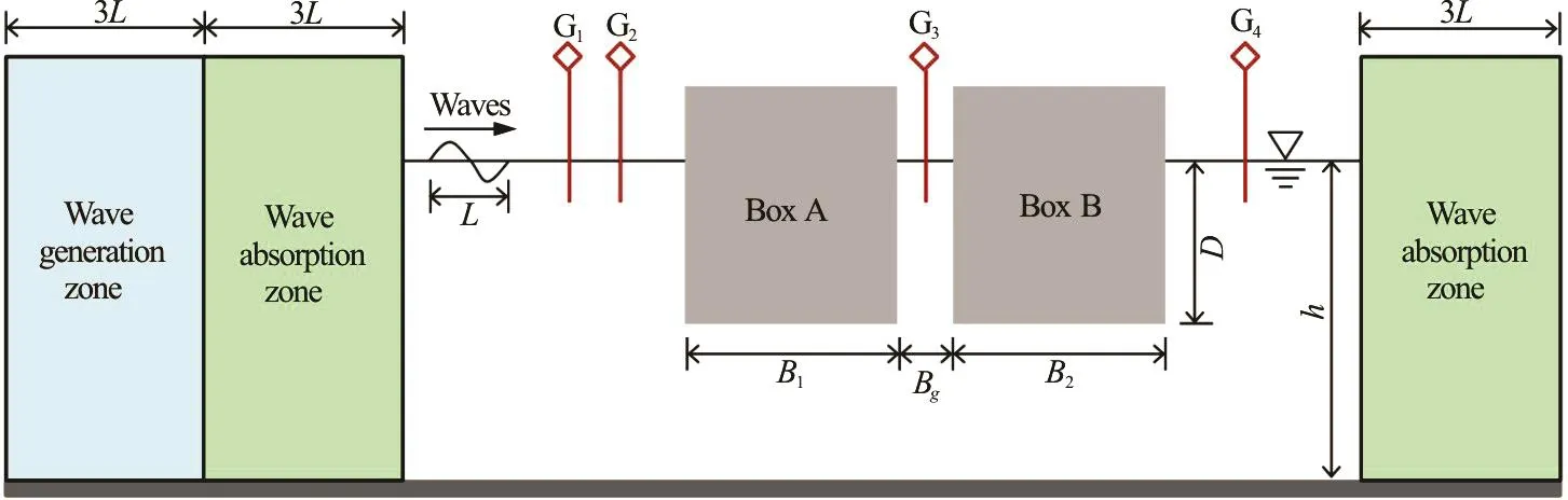
Fig.2 (Color online) Numerical setup

Fig.3(a) (Col or onlin e) Variat ions o f wave elevation RAO in gapagainstincidentwavefrequency Λ （ = ω 2Bg /g) for different breadth ratios B 2 /B1

Fig.3(b) (Color onl ine) I nfluen ce of bread th ratios on resonant frequencyandwaveelevationRAO (B1=0.50m, B g =0.05m , D =0.25m and h =0.50m)

The variations of the wave elevation RAO in the gap against the non-dimensional incident wave frequency for different box breadth ratios21/B B are shown in Fig.3(a). It can be seen that the peak value of the RAO for the smallest breadth ratio B2/B1=0.5 is about 3.8, occurring at the highest response frequency Λ = 0.146. For the case of B2/B1=1.0, the relative resonant wave amplitude is about 4.9, appearing at Λ = 0.139. As the ratio B2/B1further increases up to 1.5 and 2.0, the peak values of the RAO increase to 5.5 and 5.8,corresponding to =Λ0.138 and 0.135, respectively.It appears that the peak value of the RAO increases monotonically with21/B B. The variation of the resonant wave elevation RAO, against the resonant frequency , as a function of the breadth ratio B2/B1are presented in Fig.3(b). The relative resonant amplitude increases with the breadth ratio, as shown by the viscous numerical simulations. However,the increase rate is lower than a linear function (as shown by the dashed line in Fig.3(b)). The resonant wave frequency decreases nonlinearly with the breadth ratio21/B B, as suggested by Fig.3(b).Generally speaking, a larger breadth ratio leads to a lower resonant frequency. This can be attributed to the increase of the parameter B*with21/B B, since the present numerical simulations are conducted for a fixed1B while increasing2B.

Figure 4 presents the calculated B*/Bgvalues for different total breadths of the two boxes ( B1+ B2).The calculation is based on Eq.(15) with the obtained resonant frequency shown in Fig.3(b). It suggests that the parameter B*increases with the total breadth12+B B approximately as a linear function. Note that the natural frequency and the resonant frequency are taken as a same value in this paper since the damping coefficient ε is expected to be small.

Fig.4 (Color online) Calibrated B* /Bgvalues for different summations of box breadths (B1 + B2 )/Bg based on Eq.(15) (The resonant frequencies are based on viscous numerical simulations with B1=0.50m , Bg =0.05m , D =0.25m and h =0.50m )

Fig.5 (Color online) Variationsof relative en ergy diss ipation coefficient againstincidentwave frequency for different breadth ratios with=0.05m, D = 0.25m and h = 0.50m

Figure 5 shows the variations of the relative energy dissipation coefficient Kd(=1 -against the non- dime nsional i ncident wave frequency fordifferentboxbreadthratios B2/B1. Comparing Fig.5 with Fig.3(a), it can be found that the variation trends ofdKare generally similar to those of the RAO. The maximum values ofdKare observed to appear around the resonant frequencies.Additionally, the peak value ofdKincreases with the breadth ratio21/BB, which means that the relative energy dissipation also increases with the breadth ratio21/BB.

3.2Modified potential flow solutions

Based on the obtained results ofdKand RAO(as shown in Fig.3(a) and Fig.5), the damping coefficientpμdevised for the modified potential flow model[12,16-17]can be estimated by Eq.(32). The results are shown in Table 1. It is noted from Eq.(32)that the damping coefficientμpis dependent on the wave frequency. Nevertheless, the present numerical tests show that the modified potential flow model with a constant damping coefficientpμevaluated at the resonant condition can produce reasonable predictions for the gap resonance problem. This will further be demonstrated in the following part.

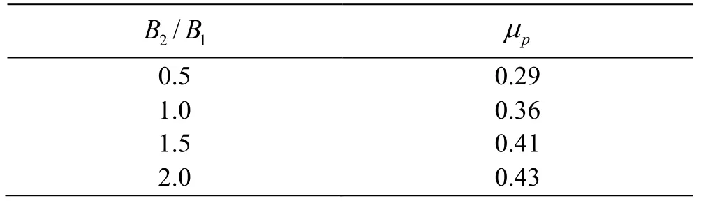
Table 1 Estimated damping coefficient μp at resonant frequency for different breadth ratios B2 /B1

The modified potential flow model, the same as that proposed by Lu et al.[16,17], is employed for predictions in the gap resonance problem with varied breadth ratios. The damping coefficientspμshown in Table 1 are used for the calculations. The corresponding modified potential solutions, including the wave elevation RAOs, the squared reflection coefficientand the transmission coefficients, for various frequencies are compared with the viscous numerical results of the RNG turbulent model in Figs.6 and 7. For the purpose of comparison, the conventional potential solutions withμp=0 are also included in Fig.6. It can be seen that the modified potential solutions (with the damping term) are in a satisfactory agreement with the viscous numerical results. It should be noticed that the dissipative effects can be completely considered by the viscous fluid model. As a contrast, the conventional potential flow model (without the damping term) leads to obvious unphysical predictions around the resonant frequency,although it works well when the wave frequency is out of a certain band around the resonant frequency.

Furthermore, as for the squared reflection and transmission coefficients (and), good agreements between the modified potential solutions(with the damping term) and the viscous numerical results are also observed, as shown in Fig.7. The good agreements observed in Figs. 6-7 confirm that (1) the relationship among the damping coefficientpμ, the response amplitude and frequency, the gap width, and the reflection and transmission coefficients, as described by Eq.(32), is reliable, (2) through the newly proposed approach, it is feasible to determine the artificial damping coefficient for the modified potential flow models without tuning it through trial tests.

4. Conclusions

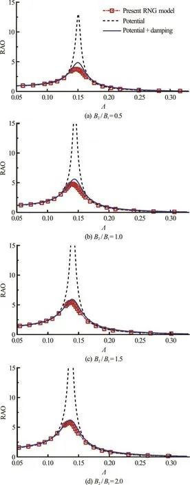
Fig.6 (Color online) Comparisons of predictions of wave eleva- tion RAO based on the potential flow model (with/without damping term) and the present RNG turbulent model for 0.05m, =0.50m different breadth ratios with =0.25m , =0.50m. Damping coe- fficient pμ is determined by Eq.(32), and is listed in Table 1

Fig.7 (Color o nline ) Comparison s of predictions ofsquar ed re- fle ction andtransmis sionco effici ents and ba sed onthepotentialflowmodelwithdampingtermandthe present RNG turbulent model for different breadth ratios with D =0.25m, =0.05m , =0.50m and h =0.50m. Damping coefficient is deter- mined by Eq. (32), and is listed in Table 1

Atheoretical dynamic model with a linearized damping coefficient is proposed for the wave resonance in a narrow gap formed by two stationary floating bodies in close proximity. With the aid of the theoretical model, the underlying relationship among the resonant response amplitude and frequency, the reflection and transmission waves, the gap width, and the damping is revealed. A quantitative link between the damping coefficient of the dynamic model (ε)and the damping coefficient devised for the modified potential models(μp) isestablished, namely,μp=3π εωn/8 (where ωnis the natural frequency).On the basis of the theoretical model and the above established link, a new approach is proposed to determine the damping coefficient for the modified potential models, without resorting to numerically tuning it through trial and error tests. The numerical results based on the modified potential flow model with the directly calculated damping coefficient are compared with the viscous numerical solutions based on the RNG turbulent model. Good agreements are obtained for the wave response in the gap, the wave reflection and the wave transmission. It is also suggested that the breadth ratio of the two floating bodies has a significant nonlinear influence on the resonant wave amplitude in the gap, the energy dissipation and the resonant frequency.

[1] Saitoh T., Miao G. P., Ishida H. Experimental study on resonant phenomena in narrow gaps between modules of very large floating structures [C]. Proceedings of International Symposiumon Naval Architecture and Ocean Engineering. Shanghai, China, 2003, 39: 1-8.

[2] Saitoh T., Miao G. P., Ishida H. Theoretical analysis on appearance condition of fluid resonance in a narrow gap between two modules of very large floating structure [C].Proceedings of the 3rd Asia-Pacific Workshop on Marine Hydrodynamics. Shanghai, China, 2006, 170-175.

[3] Molin B. On the piston and sloshing modes in moonpools[J]. Journal of Fluid Mechanics, 2001, 430: 27-50.

[4] Faltinsen O. M., Rognebakke O. F., Timokha A. N. Twodimensional resonant piston-like sloshing in a moonpool[J]. Journal of Fluid Mechanics, 2007, 575: 359-397.

[5] Yeung R. W., Seah R. K. M. On Helmholtz and higherorder resonance of twin floating bodies [J]. Journal of Engineering Mathematics, 2007, 58(1-4): 251-265.

[6] Liu Y., Li H. J. A new semi-analytical solution for gap resonance between twin rectangular boxes [J].ProceedingsInstitutionof Mechanical Engineers,Part M,2014, 228(1): 3-16.

[7] Miao G. P., Ishida H., Saitoh T. Influence of gaps between multiple floating bodies on wave forces [J]. China Ocean Engneering, 2000, 14(4): 407-422.

[8] Miao G. P., Saitoh T., Ishida H. Water wave interaction of twin large scale caissons with a small gap between [J].Coastal Engineering Journal, 2001, 43(1): 39-58.

[9] Li B., Cheng L., Deeks A. J. et al. A modified scaled boundary finite element method for problems with parallel side-faces. Part II. Application and evaluation [J]. Applied Ocean Research, 2005, 27(4-5): 224-234.

[10] Zhu H. R., Zhu R. C., Miao G. P. A time domain investigation on the hydrodynamic resonance phenomena of 3-D multiple floating structures [J]. Journal of Hydrodynamics,2008, 20: 611-616.

[11] Sun L., Eatock Taylor R., Taylor P. H. First- and secondorder analysis of resonant waves between adjacent barges[J]. Journal of Fluids Structures, 2010, 26(6): 954-978.

[12] Chen X. B. Hydrodynamics in offshore and naval applications [C]. The 6thInternational Conference onHydrodynamics. Perth, Australia, 2004.

[13] Pauw W. H., Huijsmans R., Voogt A. Advanced in the hydrodynamics of side-by-side moored vessels [C]. Proceedingsof the 26th Conference onOcean,Offshore Mechanics and ArcticEngineering (OMAE2007). San Diego, California, USA, 2007, OMAE2007-29374.

[14] Molin B., Remy F., Camhi A. et al. Experimental and numerical study of the gap resonance in-between two rectangular barges [C]. Proceedings of the 13th Congress of the International Maritime Associationof the Mediterranean (IMAM 2009). Istanbul, Turkey, 2009,689-696.

[15] Lu L., Teng B., Cheng L. et al. Modelling of multi-bodies in close proximity under water waves–Fluid resonance in narrow gaps [J]. Science China Physics Mechanics and Astronomy, 2011, 54(1): 16-25.

[16] Lu L., Teng B., Sun L. et al. Modelling of multi- bodies in close proximity under water waves–Fluid forces on floating bodies [J]. OceanEngineering, 2011, 38(13):1403-1416.

[17] Faltinsen O. M., Timokha A. N. On damping of twodimensional piston-mode sloshing in a rectangular moonpool under forced heave motions [J]. Journal of Fluid Mechanics, 2015, 772: R1, 1-11.

[18] Lu L., Cheng L., Teng B. et al. Numerical simulation and comparison of potential flow and viscous fluid models in near trapping of narrow gaps [J]. Journal of Hydrodynamics, 2010, 22(5): 120-125.

[19] Lu L., Chen X. B. Dissipation in the gap resonance between two bodies [C]. Proceedingsof the 27thInternational Workshop on Water Waves and Floating Bodies(IWWWFB 2012). Copenhagen, Denmark, 2012.

[20] Kristiansen T., Sauder T., Firoozkoohi R. Validation of a hybrid code combining potential and viscous flow with application to 3D moonpool [C]. Proceedings 32nd International Conference on Ocean, Offshore Mechanics and Arctic Engineering. Nantes, France, 2013.

[21] Fredriksen A. G., Kristiansen T., Faltinsen O. M. Waveinduced response of a floating two-dimensional body with a moonpool [J]. Philosophical Transactions of the Royal Society London A, 2015, 373(2033): 20140109.

[22] Moradi N., Zhou T. M., Cheng L. Effect of inlet configuration on wave resonance in the narrow gap of two fixed bodies in close proximity [J]. Ocean Engineering,2015, 103: 88-102.

[23] Moradi N., Zhou T. M., Cheng L. Two-dimensional numerical study on the effect of water depth on resonance behaviour of the fluid trapped between two side-by-side bodies [J]. Applied Ocean Research, 2016, 58: 218-231.

[24] Mei C. C., Stiassnie M., Yue D. K. P. Theory and applications of ocean surface waves, Part 1: Linear aspects [M].Singapore: World Scientific, 2005, 6: 285-286.

[25] Hirt C. W., Nichols B. D. Volume of fluid (VOF) method for the dynamics of free boundaries [J]. Journal of Computational Physics, 1981, 39(1): 201-225.

[26] Wang B. L., Liu H. Higher order Boussmesq-type equations for water waves on uneven bottom [J]. Applied Mathematics and Mechanics(EnglishEdition), 2005,26(6): 714-722.

Table A1 Mesh resolution for convergent test

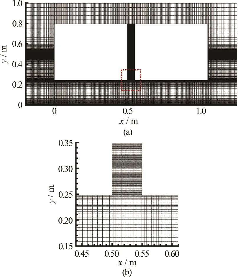
Fig.A1 (Color online) Typical computational domain computational meshes in the

Appendixes

Referring to the numerical set-up shown in Fig.2(see Page 8), the numerical convergence of the viscous fluid model is tested by five different mesh densities. Details on the mesh generations for the tested case are listed in Table A1. Mesh 1 corresponds to that, for example, the length of each mesh in -axis direction is Ai/ 12 ( Aiis the amplitude of incoming waves) near the free surface,mesh along-axis is Bg/5 length in gap, mesh along -axis is L / 10 (L is the wave length) length for the left(and right) side of the boxes, and there are 61 335 elements in total. Typical mesh partition in the computational domain is shown in Fig.A1. In order to save computational time, non-uniform meshes are adopted. In general, square fine meshes with high resolution are adopted in the gap region to account for the boundary layer effects and to accurately capture the large amplitude free surfac e oscillation.

The numericalresults ofsteady-statetime-series of the free-surface elevation in gap are compared for various mesh resolutions in Fig.A2. The comparisons indicate that the coarse Mesh 1 leads to severe numerical dissipation, while Mesh 3 is able to produce convergent solutions. And hence it is used as the baseline for the computations in this work.

The numerical accuracy of the present turbulentexperiments were carried out in a wave flume with water depth h = 0.50m. Two identical rectangular boxed with breadth B = 0.50m and draft D =0.25m were firmly arranged on the wave flume.Two gap widths were considered in the tests, i.e.,Bg=0.03 m and 0.05 m. An unchanged incident wave amplitude Ai=0.012m was adopted.

Fig.A2 (Color online) Time-seriesof free-surface elevationatprobeG3(gapcenter)withdifferent mesh resolutions (h =0.50m,B = 0.50m , D =0.25m,B =0.05m and Λ= ω 2B /g =0.139)g g

The numerical and experimental results of the variations of wave elevation RAO with the incident wave frequency Λ ( = ω2Bg/g ) are compared in Fig.A3. It shows that, for two different gap widths, the resonant frequencies are correctly predicted by the present RNG turbulent model, which are almost identical to those observed in the experiments. The variations of wave elevation RAO with frequency predicted by the present RNG turbulent model is found to be in satisfactory agreement with the experimental data.

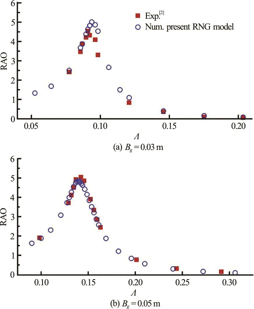
Fig.A3 (Color online) Comparisons of wave elevation RAO in gap with respect to incident wave frequency =Λ（ for twin boxes with =0.25m D, =B 0.50m and =h 0.50m

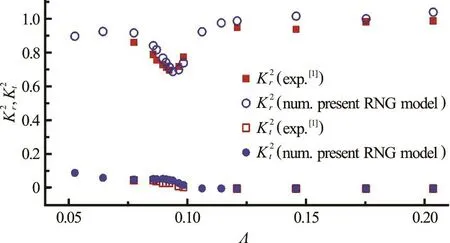
Fig.A4 (Color online) Comparisons of squared reflection and transmissio n coef ficients a nd w ith re spect to incidentwavefrequencyΛfortwinboxeswith =0.03m , D = 0.25m, B = 0.50m and h = 0.50m

The numerical and experimental results of the variations of the squared reflection and transmission coefficients,and, with the incident wave frequency are compared in Fig.A4. The experimental data for gap width=0.05m is not available, and thus no comparisons are made for=0.05m.Figure A4 shows the good agreement between the experimental data and numerical results by the present RNG model.

The comparisons shown in Figs.A3-A4 confirm that the present RNG turbulent model is able to produce accurate numerical predictions for the gap resonance problem.

June 6, 2017, Revised July 29, 2017)

* Project supported by the National Natural Science Foundation of China (Grant Nos. 51490673, 51479025 and 51279029).

Biography: Lei Tan (1989-), Male, Ph. D. Candidate

Lin Lu, E-mail: lulin@dlut.edu.cn