On the numerical simulations of vortical cavitating flows around various hydrofoils *
2017-03-14BenlongWang王本龙ZhihuiLiu刘志辉HaoyuLi李颢钰YayunWang王雅赟
Ben-long Wang (王本龙), Zhi-hui Liu (刘志辉), Hao-yu Li (李颢钰), Ya-yun Wang (王雅赟)
Deng-cheng Liu (刘登成)4, Ling-xin Zhang (张凌新)5, Xiao-xing Peng (彭晓星)4
1. Department of Engineering Mechanics, Shanghai Jiao Tong University, Shanghai 200240, China,
E-mail: benlongwang@sjtu.edu.cn
2. MOE Key Laboratory of Hydrodynamics, Shanghai Jiao Tong University, Shanghai 200240, China
3. Collaborative Innovation Center for Advanced Ship and Deep-Sea Exploration, Shanghai 200240, China
4. National Key Laboratory on Ship Vibration and Noise, China Ship Scientific Research Center, Wuxi 214082,China
5. Department of Mechanics, Zhejiang University, Hangzhou 310027, China
Introduction
Cavitation is a common physical phenomenon in many flow fields when local pressure is lower than the saturated vapor pressure, e.g., hydraulic machinery,surface ships and underwater vehicles with hydrofoils and propellers[1,2]. Stimulated by urgent need of hydrodynamic performance optimization, drag reduction and acoustic noise depression, in-depth understandings of cavitating flow characteristics are required.Accurate and effective CFD solvers can be used for scientific research and industrial applications.Verification and validation (V&V) are independent procedures that are used together to check a system of CFD simulations, which have been well expressed as:verification is a purely mathematical exercise that tends to show that we are solving the equations right,whereas validation is a science/engineering activity that tends to show that we are solving the right equations[3]. Therefore verification deals with numerical errors/uncertainties whereas validation is concerned with modelling errors/uncertainties[4].
For single-phase flows, studies of V&V have been investigated for many years[5-7]. Except for turbulence modelling, RANS model could accurately model the single-phase flows without any approximation. Therefore, validation seems to be relatively less important than verification. To the end-users of a flow solver, we could eventually obtain a converged result with mesh refinement. The point is what accuracy level we could reach with limited computational cost.For this purpose, there are several effective approaches to evaluate the uncertainty of the numerical results, if the numerical results have shown convergence trend versus mesh refinement[5,8,9]. Even though, there are some debates on the V&V approach among different works for single phase flows, such as one example around ten years ago[9,10,5]and another recent example[4,11,12].
For cavitating flows, many numerical results are strongly dependent on the mesh resolution[13], mass transfer models[14]and turbulence models[15,16], which imply either the mesh is not capable to resolve the small scale flow structures or some important flow mechanisms are not correctly modeled. Physically,many complicated flow phenomena, including the involved interface among different phases, threedimensional vortex and phase transition, have to be modelled with some kinds of approximations in cavitating flows. At this point, the validation of cavitating flows should include more themes than that of single-phase flows: such as the modellings of vapor-liquid interfaces, the discontinuities of properties across a phase interface, the mass and momentum exchange between the phases, and turbulence modelling. Although the guidelines for validation of a complex system have been established for many years[5,8,9], the whole process V&V for numerical simulations of cavitating flows is still in its infancy.
1. Numerical models
The homogeneous mixture model treats fluids in cavitating region as a mixture of two species of fluids,under assumptions of local kinematic equilibrium between phases, local thermal and mechanical properties(velocity, pressure etc.). The mixture of vapor and liquid water is treated as a single fluid, sharing the same velocity and pressure fields. The density and dynamic viscosity are evaluated depending on the void fraction of each species. Because of its simplicity,the homogeneous equilibrium mixture model is widely used for various simulations of cavitating flows. The details of numerical modelling and solving techniques for the homogeneous mixture model can be found in many references[14-16].
Mass transfer is one of the distinct physical processes for cavitating flows. To date, direct numerical simulations of evaporation and condensation are still very expansive even using massive parallel computations. To reduce the computational cost of the phase transition, mass transfer models are introduced,which will be reviewed in subsection 1.1. The detailed mechanisms of the interaction between turbulent flows and cavitation bubbles have not yet been clearly revealed, especially for phenomena occurring at small scales, unsteady or instability statuses[17,18]. Viscous effects, measured by Reynolds number, may be another important aspect of cavitating flows, which will be discussed in subsection 1.2.
1.1 Mass transfer models (cavitation models)
To describe the non-equilibrium two-phase bubbly flows, comprehensive models are required to model the physical details occurring in the cavitation phenomenon such as mass transfer, thermal transfer and surface tension. Specifically, the mass exchange between water phase and vapor phase is one of the most important processes during various cavitation phenomena. The function of volume fraction ratio can be used to track the interface between the two species.The convection of the volume fraction ratio, herein we choose the value for vapor phase, can be described as
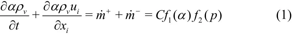
Source terms m ˙+and m˙-are the mass transfer rate between liquid water and vapor. ρvis the density of vapor, α is void fraction of vapor, and uiis velocity. Moreover, vaporization or condensation processes are assumed to be instantaneous.
Derived from the linearized Rayleigh-Plesset(R-P) equation, some cavitation models have been proposed, as listed in Table 1. In fact, it is more suitable to call these models as mass transfer models,because they occur in the terms of source and sink in the convection equation of phase function (1). As can be observed in Table 1, there are two different kinds of function2()fp: one is in the form of linear function relating to pressure difference according to the empirical formulations[19-21], the other is propor-which is a direct result of linearized R-P equation[22-24].
In principle, the linearized R-P equation cannot be used to predict the collapse of a vapor bubble.Modifications of the mass transfer model have to be introduced to improve the capability of modelling cavity collapse. In this respect, it has been shown by numerical simulations that the time histories of bubble radius for the cases of central bubble in cluster and isolated single bubble can be quite different[25,26]. This implies that there is a pronounced deficiency for the existing mass transfer models, and some modifications have to be made to improve the performance of the existing mass transfer models. The empirical coefficients in the mass transfer model have to be adjusted to meet the correct behaviors of condensation and evaporation processes. Meanwhile, the values of empirical parameters in the mass transfer model can significantly affect the stability and accuracy of the numerical simulations. Therefore, these empirical coefficients have to be calibrated with a large set of experimental data, especially for flows around new kinds of hydrofoils and propellers with complex shapes.
Since 2010s, numerous simulations have been conducted for sheet cavitating flows over hydrofoils.For NACA66(MOD) and NACA 4-digit series hydrofoils, the mass transfer models can guarantee similar levels of accuracy if the empirical parameters are properly tuned. For E779A and PPTC propellers, no significant differences were observed in the numerical simulations using the calibrated mass transfer models[27]. The optimized empirical values seem to have a good general validity[27]. However, the performance can be deteriorated in cavitating flows over complex geometries and practical operation conditions.Using the calibrated models, the cavity extension is slightly over-estimated[14,28]. The choice of the mass transfer model causes a clear difference in the thickness of the re-entrant jet[28]. For more severe operational conditions, the numerical results showed significant discrepancies with the experimental data.For rotating propellers in wake regions, it is hard to predict the dynamics of cavity region[29].
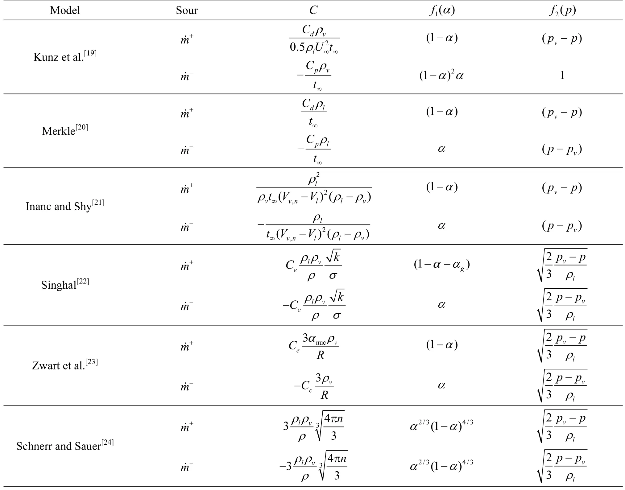
Table 1 List of cavitating models
Besides the widely used nonuniform density flow solvers, the numerical results obtained by compressible flow solvers are more encouraging. For compressible flows, the cavitation models may take different forms[17,18,30]. For both of the two compressible fluids,it contains equations for the mass, momentum and energy, and additional equation for the topology of the phase field. In the mixture area of the cavitating flows,the velocity may exceed the local sound speed and the supersonic regime occurs because of the drastic diminution of the speed of sound. The local pressure field predicted by compressible flow solvers shows different behaviors comparing that by incompressible models. Consequently, the acoustic field differs as well.
Another challenge is that the mass transfer model have to be calibrated using experimental data of cavitating flows with similar flow characteristics,which indicates that developments of more robust mass transfer models are welcome in future studies.Usually these benchmark experiments were conducted under laboratory scales. For fully developed and unsteady cavitating flows, other physical processes may influence the cavitation phenomenon besides the major scaling law relating to cavitation number. For example, thermal dynamics has been combined into the mass transfer models[31].
1.2 Turbulence models
Numerical modelling and simulations of cavita-ting flows are challenging tasks, because the flows are turbulent, highly dynamic and unstable. We do not have any general valid turbulence models yet, herein we only give a brief overview of various turbulence model strategies employed in cavitation study. For different types of turbulence cavitating flows, we need to choose one best suitable turbulence model regarding both the computational cost and accuracy.Detailed discussions will be given in specific problems.
The starting point to model the turbulence cavitating flows is the simulations using unsteady Reynolds averaged Navier-Stokes equations (RANS).In the literature, two-equation models, e.g., RNG k-ε, k-ω and SST k-ω, are frequently employed. Due to the intrinsic properties of Reynolds average operations, RANS model could capture the mean flow quantities only. More local and unsteady turbulence flow structures, and their contributions to the turbulence kinetic energy transportation, cannot be well predicted. A well-known issue is that RANS model cannot predict the shedding of cavity and more complex flows correctly.
Large eddy simulation (LES) and detached eddy simulation (DES), as a hybrid LES and RANS method,has also been used in cavitating flows, especially for unsteady and swirling flows or flows with strong separation. LES and DES can provide detailed and high fidelity velocity, pressure and their fluctuations.Therefore, direct prediction of the cavitation acoustic is possible. Most LES and DES calculations of cavitating flows follow the general routine of singlephase flows, followed the assumption of homogeneous single phase mixture. As pointed out by one recent work[16], extra stress due to fluctuations of density, velocity and void fraction has been neglected in most LES, which needs to be carefully checked comparing with detail experimental data of turbulence flows.
Besides these two categories, partial average Navier-Stokes model (PANS) is another suitable choice considering the performance and CPU cost[32].Meanwhile, it is easy to implement PANS in the existing RANS flow solvers. Time-dependent turbulent cavitating flows around a Clark-Y hydrofoil at high Reynolds number were investigated using PANS[33,34].When the tunable parameterkf, the ratio of the unresolved-to-total turbulent kinetic energy, is less than 0.5, there is a good agreement between the numerical results and experimental data on the flow structure, cavity structure and hydrodynamic loads on hydrofoil. It should be pointed out that smallerkf values require smaller mesh size and smaller time-step,tending towards the extreme limit of PANS which is DNS[35]. Consequently, the computational cost remains a major concern.
2. Sheet cavitations and cloud cavitations
2.1 Cavitating flows over NACA-series hydrofoils
Sheet cavitating flows over two-dimensional hydrofoils are one of the most fundamental studies,which has been extensively investigated in the past 15 years with the aid of CFD. During the past years,over-prediction of the turbulence eddy viscosity in the rear part of the cavity is thought to be the main reason for the poor agreement with the experimental data on cavity length, void fraction ratio and unsteady behaviors[36]. Modifications of RNG -kε model and k-ω model have been proposed for simulations of cavitating flows. Artificial reduction of eddy viscosity have been applied in many works[37]. In our early work, the influence of this kind of modification on the cavity shedding frequency had been investigated[38],comparing with the experimental results[39]and the numerical results using DES/LES. Comparisons against the numerical simulations among RANS simulations,DES and LES confirm the effects of such modification. The shedding frequency, in terms of dimensionless parameter St, could be captured in a similar value as that predicted by DES and LES for a broad range of cavitation numbers. The eddy viscosity can be depressed by 1-2 order of magnitude comparing with LES results. It should be noted that the mesh resolution, spatial scheme and the time discretization cannot help to eliminate the numerical discrepancy due to turbulence models. By detailed comparisons, it is a feasible but not a necessary approach to correctly predict the unsteady properties of shedding of cloud cavitating bubbles. In fact, this kind of artificial treatment is usually used in commercial numerical solver package, e.g., Fluent. In many open source code and homemade code, this kind of modification are not necessary.
Correct calculation of the turbulence eddy viscosity in a strict physical approach is crucial for complex cavitating flows. In framework of numerical simulations with RANS model, a nonlinear turbulence eddy viscosity model was found to be a promising approach[15], which can correctly resolve the spatial phase shift among different components of Reynolds shear stress and mean strain rate due to employing the curvature corrections, and shows distinct superiority to other turbulence models under Boussinesq assumptions. Using that numerical approach, the shedding frequency of cavitating bubble can be predicted pretty well, as shown in Fig.1. In previous studies, this kind of agreement can only be obtained by using LES[38]. It was reported that at high values of /2σα, reentrant jet dominate the shedding at Strouhal number around 0.3, while at low values of /2σα bubbly flow shock wave phenomena dominate with a Strouhal number around 0.2[40]. Using TR-PIV, a few different kinds of vortex structures have been observed in the wake region. In the viewpoint of the production and dissipation of turbulence energy, the phase lag between turbulence shear stress and mean strain rate plays an important role in modelling the turbulence dissipation for the flows with strong separation. Once more advanced turbulence models have been incorporated with the flow solvers, e.g., Reynolds stress model and DES/LES, additional modification is not necessary to eliminate the turbulence eddy viscosity[41]. The success of nonlinear turbulence eddy viscosity model and Reynolds stress model on cavitating flows implies that the classical Boussinesq assumption is not suitable for describing the relationship between strain-rate tensor and Reynolds stress tensor, especially in strong swirling flow regions and separation region. This conclusion is especially important in further studies using RANS for vortical cavitating flows.

Fig.1 Comparison of sheet cavitation shedding frequency over NACA0015 hydrofoil at different cavitation number σ and angle of attack α
2.2 Cavitating flows over twisted hydrofoils
With modern experimental techniques, 3-D sheet cavitation flow fields have been measured[42]. Since then, a lot of numerical simulations were carried out to validate the capability and reliability of DES and LES for the cavitating flows[43,44]. A more recent work on the flow structure around 3-D twisted hydrofoil has been carried out using LES with WALE SGS turbulence viscosity[16]. For =0.50 σ cascade profile collapse of cavity can be well captured using LES, in good agreements with the experimental data. Comparing with the numerical results of RANS models,more transient effects during the developing and collapse of cavity can be captured with LES.
Aiming to reduce the computational cost, the same problem is studied herein using RANS model associated with nonlinear turbulence model[15], which also serves as another validation for the proposed turbulence model. The three-dimensional twisted hydrofoil, as shown in Fig.2, has a span width of 225 mm(spanning the entire test section) and a NACA66(MOD) section with a chord length of =100 mm C

Fig.2 Illustration of the computational domain and the mesh around the NACA66 (MOD) hydrofoil
The cavity shedding processses in one cycle at σ = 1.30 are shown in Fig.3. Figure 3(a) are experimental results of the China Ship Scientific Research Center (CSSRC). The twisted hydrofoil was arranged upside down with an angle of attack α =- 2o. Two high-speed video cameras were used to record the development of cavitation region. One was put under the section to get the main view, and the other was on one side of the section to capture the side view. In Fig.3(c) almost no vapor cloud is visible in the results with the standard -kε model, also the sheet cavitation is much smaller than the experiment results in every process of cavity shedding. The results of nonlinear -kε model predict a much larger sheet cavitation region than that with the standard -kε model, and the shape of sheet cavitation matches better with the experiment results. What’s more, in the results with the nonlinear -kε model an apparent vapor cloud is captured almost in the same location as that in the experiment results. The results of nonlinear k-ε model match better with the experiment results than that of standard -kε model in both sheet and cloud cavitating regions. A U-shape vapor cloud behind the sheet cavitation can be resolved using nonlinear -kε model as shown in Fig.3(b). Also, the same kinds of structures have been observed in the previous experimental studies[42]. In contrast, there is no such kinds of U-shape structure in the results with the standard -kε model in Fig.3(c).
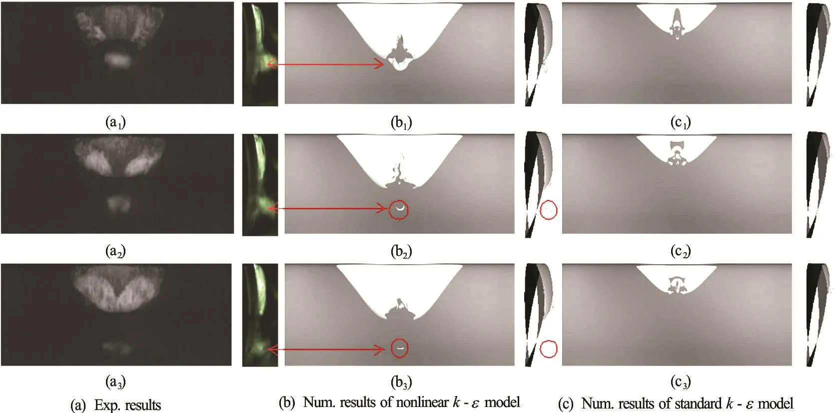
Fig.3 (Color online) Top and side views of cavity shedding processes for σ=1.30 for both experiment results of CSSRC and numerical simulations (α v=0.5for numerical results)

Fig.4 (Color online) The relationship between cavity structures and vortical structures, numerical results with the nonlinear k -ε model at σ =1.30
Vortical structures can be predicted according to the nonlinear -kε model as shown in Fig.4. When increasing the value of Q-criterion from Q =5× 10⁵to Q = 2× 1 06, the simulation with nonlinear k -ε model shows a region of high level of vorticity,especially in the flow separation region. The vortex cavitation will happen when the vortex is strong enough to generate a low enough pressure below saturated vapor pressure in the core of the vortex. As there is no such high level of vorticity in the separation region predicted by the standard -kε model in Fig.3(c), there is no vapor cloud behind the sheet cavitation.
In Fig.4 hairpin-shape vortices are found in both the end of sheet cavitation and the separation region.By comparing the vortices structure in Fig.4(b) and Fig.4(c), we can see that the hairpin-shape vortex structure has developed into a U-shape vortex structure by leaving the two legs attached to the wall.So we speculate that the U-shape cavitating vortex structure develops from hairpin-shape vortices.
Two different kinds of turbulence models are used in this study with the same mesh resolution. By comparing the numerical results based on those two different kinds of turbulence models, the simulations with nonlinear -kε model can predict longer sheet cavitation and more clear U-shape cloud cavitation.Also, the numerical results based on nonlinear -kε model match better with the experimental results.According to the numerical results, we can observe that the vortex structure plays a crucial role in the prediction of the unsteady characteristic of the cavitation flow around the three-dimensional twisted hydrofoil. As illustrated, the nonlinear -kε model is a promising candidate for predicting unsteady cavitation flow by reducing the dissipation in the vortex region at a relative low computational cost.
2.3 Tip vortex cavitating flows
Tip vortex cavitating flows is one typical vortical cavitating flows. Flow separation and swirling are two major characteristics in tip vortex cavitating flows.Two kinds of numerical dissipations may affect the numerical simulation accuracy of tip vortex cavitating flows. The first one comes from the mesh resolution,which is sensitive in capturing the tip vortex cavitating flows. With a local refined block along the helix line,the cavities in the tip, root and leading edge can reasonably be captured[15]. Another kind of the numerical dissipation comes from the turbulence models. The phase shift between the Reynolds shear stress tensor and mean strain rate tensor may significantly reduce the dissipation of turbulence energy. Therefore, the nonlinear turbulence model may aid to improve the accuracy of the cavitating simulations. Because of the importance of turbulence dissipation, we suggest that such kind of comparison between Reynolds shear stress tensor and mean strain rate tensor should be taken as a critical benchmark for numerical models of vortical cavitating flows. More details on the numerical results obtained using RANS model can refer to the early work[15].
For hydrofoils of simple geometry, DES or LES is applicable for academic study. For practical applications, acoustic noise is an important quantity.Therefore, fluctuation of pressure is an important output for the numerical simulations. Fluctuations of velocity and pressure can only be obtained using either DES or LES. We perform DES for both fully wet and cavitating flows over a truncated NACA0015 hydrofoil of aspect ratio AR=1, following the same numerical procedures in early work[38]. Using local mesh refinement in the tip vortex region, the total grid number is around 1.1×10⁷, as shown in Fig.5. The origin =0x locates at the leading edge of the hydrofoil. There are around 5 000 computational cells in the vortex region. Therefore, a triple vortex structure and their merging process could be well resolved in a similar manner as observed in experiments[45]. As shown in Fig.6, a detached tip vortex cavitation bubble, due to the strengthen of the local vorticity during the merging process, has been captured for the simulated case =1.00σ. Similar phenomenon has been recorded in experiments as well[46]. It is observed that the location of both visual inception and the first sub-visual citation events is around 1/2 to 1 chord length of the blade[47,48], which cannot be well explained according to the dynamics of nucleation bubbles.
Fig.5 (Color online) Refinement of the computational grid in the vicinity of tip and vortex center region
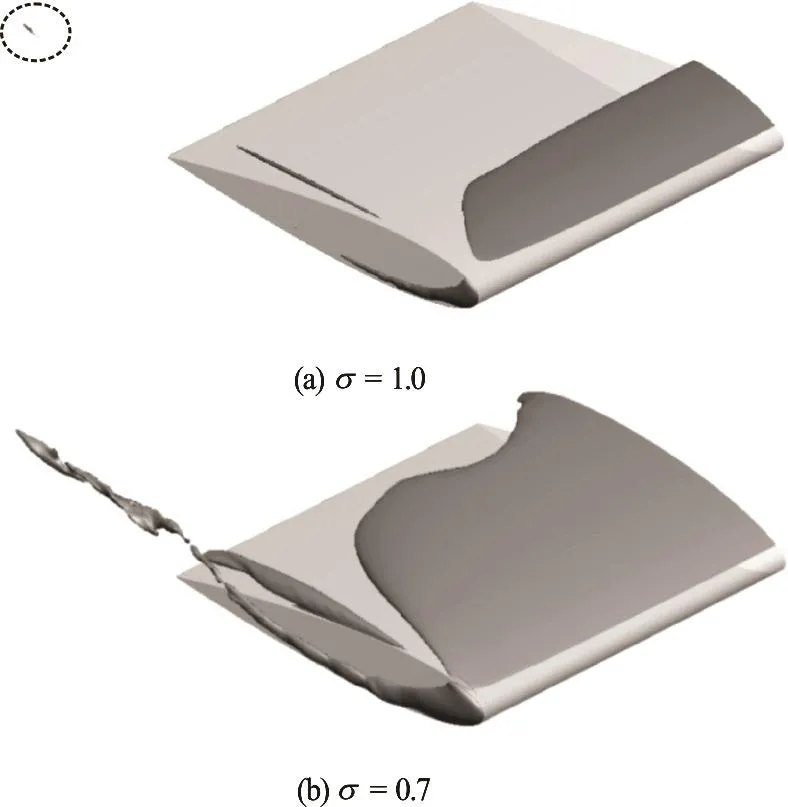
Fig.6 Instantaneous iso-surface of volume fraction function.Parameters: R e = 4.6× 10⁶, α =10o, σ=1.00
At Re = 4.6× 10⁶and σ = 0.70, the magnitude of dimensionless pressure fluctuation can reach 0.03 as shown in Fig.7. Meanwhile, the dimensionless fluctuation velocity isaround 0.1-0.2, which is insimilarmagnitudeasthe experimental Comparing with the saturated vapor pressure, the pressure fluctuation due to turbulence is an important factor in numerical simulations of cavitating flows,especially for cavitation inception and desinence. This is the reason why the unsteadiness effects due to turbu-lence are incorporated into the inception scaling law[50]. As can be observed in Fig.7, there are a few very small, intense vortices which generate very low pressure. These strong vortices seem to be responsible for the discrete tip-vortex cavitation

Fig.7 (Color online) Normalized RMS pressure fluctuations C p′= p ′/(1 / 2ρ ) at different planes along a NACA0015 hydrofoil, DES results
2.4 Tip leakage vortex cavitating flows
When the tip of a hydrofoil is located close to a solid wall, the tip vortex is confined in a narrow gap region, which is termed as tip leakage or tip clearance flows. The tip leakage flows are important topics in rotating machineries such as axial pump impellers and ducted propellers, which have been extensively studied in different fields[51-62]. Due to the sharp difference between the chordwise pressure gradients and the normal pressure gradients in the clearance region, the tip clearance flows can be approximately decomposed into independent through-flow and crossflow[63], which provide a theoretical basis to simplify the complex flows in rotating machineries. Neglecting the chordwise rotating flows inside a casing, flow around a hydrofoil near a plate with a narrow gap is a simple model for both experimental and numerical studies, which provides the most important characteristics of tip leakage flows.
Different flow regime in the tip leakage flows are illustrated in Fig.8. Clearly, there are two different types of flows: strong tip vortex cavitating flow relating to cavitation number σ, separation flows at the edge of the hydrofoil’s tip relating to Reynolds number Re. To quantitatively describe the tip leakage flow, both of these two kinds of flows should be properly simulated. Besides the general requirements for the tip vortex cavitating flows as mentioned in Section 3, the interactions between the separation bubble and the wall boundary layer, which depends heavily on the Reynolds number, is another crucial issue for the numerical simulations.
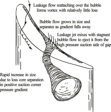
Fig.8 Sketch of flow phenomenon in the gap region, reproduced following Bindon[51]
The unsteady, secondary vortical structures were expected to be the trigger mechanism for tip-leakage vortex cavitating inception. Therefore, advanced numerical models, especially the turbulence models, are among the critical factors to predict the inception.Indeed, it is far away from predicting inception numerically.
Herein, the flows around a truncated NACA0009 hydrofoil have been simulated with RANS equations and the nonlinear -kε turbulence model[15]. The setup follows the water tunnel experiments[64]. The hydrofoil is mounted on a vertical plate with an angle of attack α = 11o. There is a gap between the free end and the vertical plate. The incoming velocity is 10 m/s and the corresponding Reynolds number is =Re 1.0× 10⁶, and the cavitation number is σ=1.94.
The gap size τ, usually normalized by the maximum thickness of the hydrofoil, has a significant influence on the tip-leakage vortex cavitating flows.Numerical simulations with various dimensionless gap size τ are conducted. One example of numerical results is shown in Fig.9. Both cases of gap size smaller and larger than the plate boundary thickness are investigated. According to the measurements of the cavitation flows around a 3-D NACA0009 hydrofoil by using stereo-PIV, it was found that there exist a specific tip clearance for which the vortex strength is maximum and most prone to generating cavitation[64]. It was found that the strongest tipleakage cavitation occurs near =0.2τ. From the numerical study we found that the boundary layer on the side plate near the free end of the hydrofoil plays an important role in the upward tendency of the tip-leakage vortex. When the free end is inside the boundary layer, there is an obvious upward tendency of the vortex structure. It was observed that the tip leakage vortex trajectory moves closer to the hydrofoils as the clearance is increased in early experimental study[54]. The meandering of the vortex core is substantial in the experiments, but have not been predicted in present numerical simulations.

Fig.9 (Color online) Comparisonon the numerical resultsandinstantaneousexperimentalhigh-speed τ=0.7
An empirical law that matches the vortex trajectory from the leading edge to the mid-chord has been proposed based on the numerical results on a noncavitating tip-leakage flow around NACA0009 hydrofoil[66]. From the present numerical results, there is a difference in the trajectories of cavitating and noncavitating tip-leakage vortex flows, as shown in Fig.10, when the dimensionless gap size is smaller than 1.0. This kind of difference deserves to be investigated in future studies, which will help to establish an empirical law for the vortex trajectories in the cavitating tip-leakage flows.
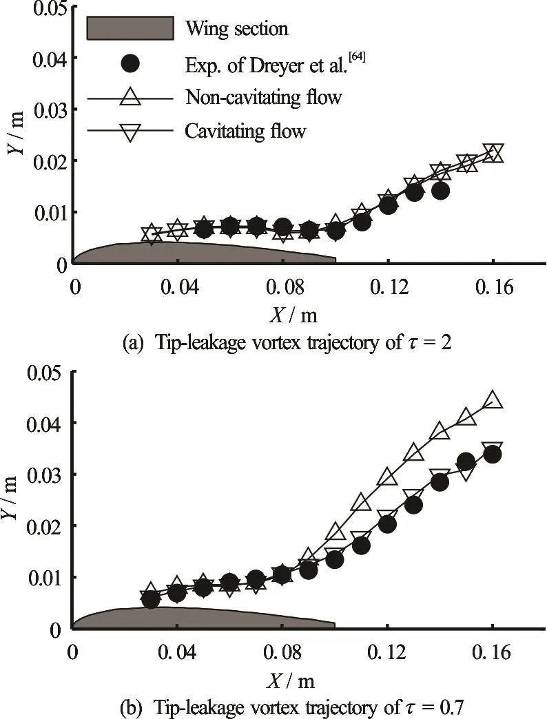
Fig.10 Comparison on the trajectories of cavitating and noncavitating tip-leakage vortex flows[65]
Several early papers have dealt with the cavitation in tip leakage or tip clearance flows. The location of the cavitating vortex origin moved along the streamwise direction, depending on the relative gap size τ[52]. The influence of Reynolds number among experiments is smaller than the general propellers and hydrofoils in open water. The measured dependence on inception number for the propulsor is 0.21[55],which is significantly lower than the empirical values 0.3[52], or 0.4-0.5[50]. The visual inception and the sub-visual cavitation events occur approximately at the merge location of tip-leakage vortex and trailing edge vortex. Careful investigations on the merging process may help to resolve the mismatch between the lowest pressure location and inception location.Several relevant works have been conducted recently for two co-rotating vortices[67,68]. Extension of these works for cavitating flows should be another important aspect of fundamental research.
When there is no relative motion between the tip and the end wall, experiments do not show a minimum in the cavitation inception index[53,54], which is diffe-rent from the experience obtained from the experiments for a rotating turbomachine[52]. Before ending this section, it should be emphasized that simulations of 3-D cavitating tip-leakage flow field around rotators are important to understand the realistic flow field in turbomachinery. A few 3-D RANS simulations, using SST -kω and other two-equation turbulence models, have been conducted for the full rotation machinery recently[62,69], in which flow rate and TLV trajectory can be quantitatively predicted.Using LDV and PIV, detailed tip-leakage flow fields inside ducted propulsors at Reynolds number 106have been measured[56,57]. Comparisons on the turbulence flow field with these experimental results are important and challenging tasks, which require high computational efforts as well as accurate cavitation models and turbulence models[70].
3. Remarks and outlook
This paper reviewed the achievements of various numerical results on cavitating flows around hydrofoils in recent years. For practical applications,various RANS solvers have the capabilities to predict the steady cavitating flows. On account of instantaneous flow fields and fluctuations, DES and LES seem to be the promising approaches. Generally,numerical simulations of sheet cavitation over various hydrofoils are successful today. For cloud cavitating flows, tip vortex and leakage vortex cavitating flows,there are a lot of fundamental flow mechanisms to be identified. In many circumstances, it is important to investigate the unsteady cavitating flow phenomena,such as cavitation inception, instability and burst.Laboratory experiments seem to be the first choice to identify and grasp the concealed flow mechanisms.More fundamental experimental research works have to be conducted to establish a deep understanding of the local flow structures and the property of vaporwater mixture. Once these flow characteristics inside the local region are known, more elaborate mathematical models and numerical flow solvers can be developed.
Although significant improvements have been obtained in the past years, there is still a large gap between the academic studies and industrial applications. Several tasks are urgently to be carried out:large scale parallel simulations, numerical models for shedding and collapse of the cloud cavitation, simulations of the behavior of tip leakage cavitating flows and acoustic noise estimation etc.. In future studies,there are several open questions deserving to be further investigated:
(1) Can mass transfer model originated from Rayleigh-Plesset equation predict cavity collapse and more general bubbly-like cavitating flows? The mass transfer models summarized in Section 1 are based on linearized R-P equation. The transient effects are profound in the collapse process, and the absent of nonlinear effects is one of the main flaws. Although some numerical models with advanced turbulence models can correctly capture the large scale collapse of cavitating region, the detailed distribution of two phases fluids and velocity in the cloud cavitation region still cannot be well simulated. Besides the mass transfer model, interactions among a large number of bubbles could be another important reason. Direct numerical simulations of the behavior of bubble clusters[25,26], accompanied by fundamental experiments, can help to tune the parameters in the mass transfer model. As the bubble size may vary significantly in realistic situations, there should be some multiform and multiscale numerical models depending on the background mesh size, to distinguish the dynamics of different size bubbles.
(2) Besides homogeneous mixture model, are there any other suitable models for numerical simulations of cavitating flows? There are several new and instructive experimental results on the flow structures,cavitation bubble interface and vapor bubble size distribution inside the cavitation region[40,71,72], which is not easy to be correctly predicted using homogeneous mixture model. The effects of gas/vapor content,surface characteristics, and system stability become especially important in actual applications. For example, Euler-Lagrangian coupled method seems to be a promising approach for high fidelity multiphase flow simulations, especially for tip vortex cavitation and cavitation inception[73-75]. Using Lagrangian method, the motions of vapor bubbles of size much smaller than grid size can be well predicted, and consequently the influence of the bubble size spectrum can be investigated.
(3) Can the simplified mass transfer model deteriorate the high fidelity flow field obtained from DES and LES? The main challenge is to establish an enhance mass transfer model with equal accuracy as high fidelity flow fields. Various DES and LES have been verified to be valid and accurate approaches in many different kinds of flows, although additional averaging have to be conducted for varying density flows such as compressible flows and multiphase flows[76]. However, the mass transfer models in many DES and LES of cavitating flows directly succeed the ones used in RANS simulations. The correlation between the fluctuation of phase function and velocity fluctuations lacks carefully examinations. Additional effects may occur in both the momentum equations and transportation equation of phase function.
(4) How to establish a robust and compatible cavitating model which can treat various cavitation processes, including sheet cavitation, cloud cavitation and vortical cavitation coinstantaneously? As a first step, many numerical models are investigated only for one specified type of cavitating flows. In realistic applications, various cavitation phenomenon usually occur simultaneously. Due to the distinct difference on generation mechanisms, it is speculated that one threshold, usually taken as saturated vapor pressure, is not suitable for different cavitating processes.
(5) How to perform V&V of numerical simulations of cavitating flows, especially for LES? With the fast development of computational hardware, LES becomes much more popular recently. An instructive and thorough framework of V&V for a general cavitating flow solver has been proposed and established using RANS models and LES respectively[77,78].However, V&V of LES for cavitating flows needs special considerations. Similar to dispersal bubbly flows, micro-, meso-, and macroscales of cavitating flows need different numerical models[78,79]. Mesoscales studies are expected to be ideal modes and can be carried out at reasonable computation costs.Physically, the size of the vapor bubbles inside cloud cavitation region varies from tens of microns to several millimeters, which is comparable with the filter length or mesh size in high fidelity meso-scale LES. Some flow models, especially for homogeneous mixture models, are not valid for statistical description of the bubbles of such size distributions. In recent years, it seems to be more important to perform the validation analysis, specifically for the multiphase flow model, mass transfer model and turbulence model. Research should take special cares in order to solve the equations describing the underlying physics consistently.
Meanwhile, due to the overlap of vapor bubble size, meso-flow scale and filter length, it is not suitable for conducting general quantitative estimations of numerical error and the associated uncertainties by mesh convergence investigations. The most likely verifications of LES SGS models may be performed through a priori analysis of direct numerical simulation data[25,26], and a posteriori analysis of LES results via comparison with the laboratory experiments. Benchmark experiments are particularly important to validate these numerical models[39,42,46,64,80]. A few important databases for various benchmark cavitating flows were released by CSSRC and SJTU recently[71,72,81], which includes many details of flow structures, properties of multiphase fluid and multiphysics problems, and will significantly expand the databases for V&V. As various cavitating flows involve sophisticated flow mechanisms and the numerical modelling on them remains an immature research field, fundamental and elaborately experimental studies should be the first choice to identify the flow characteristics and mechanism, and will play important roles in validating the numerical models.
Acknowledgement
Thanks for the discussions and exchange of academic thoughts in the series mini-symposiums of cavitating flows during the past 8 years, organized by China Ship Scientific Research Center, Zhejiang University, Shanghai Jiao Tong university, Marine Design and Research Institute of China and Wuhan University.
[1] Zhang L. X., Zhang N., Peng X. X. et al. A review of studies of mechanism and prediction of tip vortex cavitation inception [J]. Journal of Hydrodynamics, 2015, 27(4):488-495.
[2] Luo X. W., Ji B., Tsujimoto Y. A review of cavitation in hydraulic machinery [J]. Journal of Hydrodynamics, 2016,28(3): 335-358.
[3] Roache P. J. Verification and validation in computational science and engineering [M]. Albuquerque, New Mexico,USA: Hermosa Publishers, 1998.
[4] Eca L., Hoekstra M. A procedure for the estimation of the numerical uncertainty of CFD calculations based on grid refinement studies [J]. Journal of Computational Physics,2014, 262: 104-130.
[5] Stern F., Wilson R., Shao J. Quantitative V&V of CFD simulations and certification of CFD codes [J]. International Journal for Numerical Methods in Fluids, 2006,50(11): 1335-1355.
[6] Zhang Z. R. Verification and validation for RANS simulation of KCS container ship without/with propeller [J].Journal of Hydrodynamics, 2010, 22(5Suppl.): 932-939.
[7] Zou L., Larsson L., Orych M. Verification and validation of CFD predictions for a manoeuvring tanker [J]. Journal of Hydrodynamics, 2010, 22(5Suppl.): 438-445.
[8] AIAA. Guide for the verification and validation of computational fluid dynamics simulations [R]. Reston, VA, USA:American Institute of Aeronautics and Astronautics, 1998,AIAA-G-077-1998.
[9] Oberkampf W. L., Trucano T. G. Verification and validation in computational fluid dynamics [J]. Progress in Aerospace Sciences, 2002, 38: 209-272.
[10] Roache P. J. Criticisms of the correction factor verification method [J]. Journal of Fluids Engineering, 2003, 125(4):732-733.
[11] Xing T., Stern F. Comment on “A procedure for the estimation of the numerical uncertainty of CFD calculations based on grid refinement studies” (L. Eca and M. Hoekastra,Journal of Computational Physics 262(2014)104-130) [J].Journal of Computational Physics, 2015, 301: 484-486.
[12] Eca L., Hoekstra M. Reply to comment on “A procedure for the estimation of the numerical uncertainty of CFD calculations based on grid refinement studies” (L. Eca and M. Hoekastra, Journal of Computational Physics 262(2014)104-130) [J]. Journal of Computational Physics,2015, 301: 487-488.
[13] Long Y., Long X. P., Ji B. et al. Verification and validation of URANS simulations of the turbulent cavitating flow around the hydrofoil [J]. Journal of Hydrodynamics,2017, 29(4): 610-620.
[14] Morgut M., Nobile E. Numerical predictions of cavitating flow around model scale propellers by CFD and advanced model calibration [J]. International Journal of Rotating Machinery, 2012, 618180.
[15] Liu Z. H., Wang B. L., Peng X. X. et al. Calculation of tip vortex cavitation flows around three-dimensional hydrofoils and propellers using a nonlinear -kε turbulence model [J]. Journal of Hydrodynamics, 2016, 28(2):227-237.
[16] Chen Y., Chen X., Li J. et al. Large eddy simulation and investigation on the flow structure of the cascading cavitation shedding regime around 3D twisted hydrofoil[J]. Ocean Engineering, 2017, 129: 1-19.
[17] Goncalvès E., Charrière B. Modeling for isothermal cavitation with a four-equation model [J]. International Journal of Multiphase Flow, 2014, 59: 54-72.
[18] Ha C. T., Park W. G. Evaluation of a new scaling term in preconditioning schemes for computations of compressible cavitating and ventilated flows [J]. Ocean Engineering, 2016, 126: 432-466.
[19] Kunz R. F., Boger D. A., Stinebring D. R. et al. A preconditioned Navier-Stokes method for two-phase flows with application to cavitation prediction [J]. Computers and Fluids, 2000, 29(8): 849-875.
[20] Merkle C. L., Feng J., Buelow P. E. O. Computational modeling of the dynamics of sheet cavitation [C].Proceedings of the 3rd International Symposium on Cavitation. Grenoble, France, 1998.
[21] Inanc S., Shy W. Interfacial dynamics-based modeling of turbulent cavitating flows, Part-Ι: Model development and steady-state computations [J]. International Journal for Numerical Methods in Fluids, 2004, 44(9): 975-995.
[22] Sinhal A. K., Athavale M. M., Li H. et al. Mathematical basis and validation of the full cavitation model [J].Journal of Fluids Engineering, 2002, 124(3): 617-624.
[23] Zwart P. J., Gerber A. G., Belamri T. A two-phase flow model for predicting cavitation dynamics [C]. Fifth International Conference on Multiphase Flow. Yokohama,Japan, 2004.
[24] Schnerr G. H., Sauer J. Physical and numerical modeling of unsteady cavitation dynamics [C]. Proceeding of the 4th International Conference on Multiphase Flow. New Orleans, La, USA, 2001.
[25] Zhang L. X., Yin Q., Shao X. M. Theoretical and numerical studies on the bubble collapse in water [J]. Chinese Journal of Hydrodynamics, 2012, 27(1): 68-73(in Chinese).
[26] Chen Y., Lu C. J., Chen X. et al. Numerical investigation of the time-resolved bubble cluster dynamics by using the interface capture method of multiphase flow approach [J].Journal of Hydrodynamics, 2017, 29(3): 485-494.
[27] Morgut M., Nobile E., Bilus I. Comparison of mass transfer models for the numerical prediction of sheet cavitation around a hydrofoil [J]. International Journal of Multiphase Flow, 2011, 37(6): 620-626.
[28] Salvatore F., Streckwall H., van Terwisga T. Propeller cavitation modelling by CFD-results from the VIRTUE 2008 Rome workshop [C]. First International Symposium on Marine Propulsors. Trondheim, Norway, 2009.
[29] Liu D. C., Zhou W. X. Numerical predictions of the propeller cavitation behind ship and comparison with experiment [J]. Journal of Ship Mechanics, 2016, 20(3):233-242.
[30] Goncalvès E. Modeling for non-isothermal cavitation using 4-equation models [J]. International Journal of Heat and Mass Transfer, 2014, 76: 247-262.
[31] Zhang Y., Luo X., Ji B. et al A thermodynamic cavitation model for cavitating flow simulation in a wide range of water temperatures [J]. Chinese Physics Letters, 2010,27(1): 016401
[32] Girimaji S., Abdol-Hamid K. S. Partially averaged Navier Stokes model for turbulence: Implementation and validation [C]. 43rd AIAA Aerospace Sciences Meeting and Exhibit. Reno, Nevada, 2005.
[33] Huang B., Wang G. Y. Partially averaged Navier Stokes method for time-dependent turbulent cavitating flows [J].Journal Hydrodynamics, 2011, 23(1): 26-33.
[34] Ji B., Luo X. W., Wu Y. L. et al. Partially-averaged Navier-Stokes method with modified -kε model for cavitating flow around a marine propeller in a nonuniform wake [J]. International Journal of Heat and Mass Transfer, 2012, 55(23): 6582-6588.
[35] Lakshmipathy S. Partially averaged Navier-Stokes method for turbulence closures: characterization of fluctuations and extension to wall bounded flows [D]. Doctoral Thesis,2009, College Station, USA: Texas A&M University.
[36] Coutier-Delgosha O., Fortes-Patella R., Reboud J. L. Evaluation of the turbulence model influence on the numerical simulations of unsteady cavitation [J]. Journal of Fluids Engineering, 2003, 125(1): 38-45.
[37] Chen Y., Lu C. J., Wu L. Modelling and computation of unsteady turbulent cavitation flows [J]. Journal of Hydrodynamics, 2006, 18(5): 559-566.
[38] Wang Y. Y., Wang B. L., Liu H. Numerical simulation of sheet cavity shedding and cloud cavitation on a 2D hydrofoil [J]. Chinese Journal of Hydrodynamics, 2014,29(2): 175-182(in Chinese).
[39] Kjeldsen M., Arndt R. E. A., Effertz M. Spectral characteristics of sheet/cloud cavitation [J]. Journal of Fluids Engineering, 2000, 122(3): 481-487.
[40] Arndt R. E. A. Some remarks on hydrofoil cavitation [J].Journal of Hydrodynamics, 2012, 24(3): 305-314.
[41] Frank T., Lifante C., Jebauer S. et al. CFD simulation of cloud and tip vortex cavitation on hydrofoils [C]. 6th International Conference on Multiphase Flow ICMF.Leipzig, Germany, 2007.
[42] Foeth E. J., Van Doorne C. W. H., Van Terwisga T. et al.Time resolved PIV and flow visualization of 3D sheet cavitation [J]. Experiments in Fluids, 2006, 40(4):503-513.
[43] Schnerr G. H., Sezal I. H., Schmidt S. Numerical investigation of three-dimensional cloudy cavitation with special emphasis on collapse induced shock dynamics [J]. Physics of Fluids, 2008, 20(4): 040703.
[44] Ji B., Luo X. W., Peng X. X. et al. Three-dimensional large eddy simulation and vorticity analysis of unsteady cavitating flow around a twisted hydrofoil [J]. Journal of Hydrodynamics, 2013, 25(4): 510-519.
[45] Bailey S. C. C., Tauvolaris S., Lee B. H. K. Effects of free-stream turbulence on wing-tip vortex formation and near field [J]. Journal of Aircraft, 2006, 43(5): 1282-1291.[46] Arndt R. E. A., Arakeri V. H., Higuchi H. Some observations of tip-vortex cavitation [J]. Journal of Fluid Mechanics, 1991, 229: 269-289.
[47] Brewer W. H. On simulating tip-leakage vortex flow to study the nature of cavitation inception [D]. Doctoral Thesis, Starkville, USA: Mississippi State University,2002.
[48] Christopher J. C., Stuart D. J. Tip-vortex induced cavitation on a ducted propulsor [C]. 4th ASME-JSME Joint Fluids Engineering Conference. Honolulu, Hawaii, USA,2003.
[49] Chow J. S., Zilliac G. G., Bradshaw P. Mean and turbulence measurements in the near field of a wingtip vortex[J]. AIAA Journal, 1997, 35(10): 1561-1567.
[50] Arndt R. E. A. Cavitation in vortical flows [J]. Annual Review of Fluid Mechanics, 2003, 34(1): 143-175.
[51] Bindon J. P. The measurement and formation of tip clearance loss [J]. Journal of Turbomachinery, 1989, 111(3):257-263
[52] Farrell K. J., Biller M. L. A correlation of leakage vortex cavitation in axial-flow pumps [J]. Journal of Fluids Engineering, 1994, 116(3): 551-557.
[53] Boulon O., Callenaere M., Franc J. P. et al. An experimental insight into the effect of confinement on tip vortex cavitation of an elliptical hydrofoil [J]. Journal Fluid Mechanics, 1999, 390: 1-23.
[54] Gopalan S., Katz J., Liu H. L. Effect of gap size on tip leakage cavitation inception, associated noise and flow structure [J]. Journal of Fluids Engineering, 2002, 124(4):994-1004.
[55] Chesnakas C. J., Jessup S. D. Tip-vortex induced cavitation on a ducked propulsor [C]. Proceedings of ASME FEDSM’03, 4th ASME_JSME Joint Fluids Engineering Conference. Honolulu, Hawaii, USA, 2003.
[56] Oweis G. F., Fry D., Chesnakas C. J. et al. Development of a tip-leakage flow-Part 1: The flow over a range of Reynolds numbers [J]. Journal of Fluids Engineering,2006, 128(4): 751-764.
[57] Oweis G. F, Fry D., Chesnakas C. J. et al. Development of a tip-leakage flow-Part 2: Comparison between the ducted and un-ducted rotor [J]. Journal of Fluids Engineering,2006, 128(4): 765-773.
[58] Wu H., Miorini R. L., Katz J. Measurements of the tip leakage vortex structures and turbulence in the meridional plane of an axial water-jet pump [J]. Experiments in Fluids, 2011, 50(4): 989-1003.
[59] Wu H., Tan D., Miorini R. L. et al. Three-dimensional flow structures and associated turbulence in the tip region of a waterjet pump rotor blade [J]. Experiments in Fluids,2011, 51(6): 1721-1737.
[60] Wu H., Miorini R. L., Tan D. et al. Turbulence within the tip-leakage vortex of an axial waterjet pump [J]. AIAA Journal, 2012, 50(11): 2574-2587.
[61] Miorini R. L., Wu H., Katz J. The internal structure of the tip leakage vortex within the rotor of an axial waterjet pump [J]. Journal of Turbomachinery, 2012, 134(3):403-419.
[62] Zhang D., Shi W., Pan D. et al. Numerical and experimental investigation of tip leakage vortex cavitation patterns and mechanism in an axial flow pump [J].Journal of Fluids Engineering, 2015, 137(12): 815-816.
[63] Chen G. T., Gretzer E. M., Tan C. S. et al. Similarity analysis of compressor tip clearance flow structure [J].Journal of Turbomachinery, 1991, 113(2): 260-269.
[64] Dreyer M., Decaix J., Munch-Alligne C. et al. Mind the gap: A new insight into the tip leakage vortex using stereo-PIV [J]. Experiments in Fluids, 2014, 55(11): 1-13.[65] Liu Z. H., Wang B. L. RANS simulations of tip leakage vortex cavitation flows around NACA0009 hydrofoil [C].Fifth International Symposium on Marine Propulsors smp’17. Espoo, Finland, 2017.
[66] Decaix J., Balarac G., Dreyer M. et al. RANS and LES computations of the tip leakage vortex for different gap widths [J]. Journal of Turbulence, 2015, 16(4): 309-341.
[67] Josserand C., Rossi M. The merging of two co-rotating vortices: A numerical study [J]. European Journal of Mechanics B/Fluids, 2007, 26(6): 779-794.
[68] Delbende I., Piton B., Rossi M. Merging of two helical vortices [J]. European Journal of Mechanics B/Fluids,2015, 49: 363-372.
[69] Zhang D., Shi W., Esch B. P. M. et al. Numerical and experimental investigation of tip leakage vortex trajectory and dynamics in an axial flow pump [J]. Computers and Fluids, 2015, 112(1): 61-71.
[70] Hah C. Effects of double-leakage tip clearance flow on the performance of a compressor stage with a large rotor tip gap [J]. Journal of Turbomachinery, 2017, 139(6): 061006.
[71] Peng X. X., Ji B., Cao Y. T. et al. Combined experimental observation and numerical simulation of the cloud cavitation with U-type flow structures on hydrofoils [J].International Journal of Multiphase Flow, 2016, 79:10-22.
[72] Wan C., Wang B., Wang Q. et al. Probing and imaging of vapor-water mixture properties inside partial/cloud cavitating flows [J]. Journal of Fluid Engineering, 2017,139(3): 031303.
[73] Fuster D., Colonius T. Modelling bubble clusters in compressible liquids [J]. Journal Fluid Mechanics, 2011, 688:352-389.
[74] Chahine G. L., Hsiao C. T., Raju R. Scaling of cavitation bubble cloud dynamics on propellers [M]. Chapter 15 in Advanced experimental and numerical techniques for cavitation erosion prediction. Dordrecht, The Netherlands:Springer, 2014.
[75] Zhang L., Chen L., Shao X. The migration and growth of nuclei in an ideal vortex flow [J]. Physics of Fluids, 2016,28(12): 123305.
[76] Fox R. O. Large-eddy-simulation tools for multiphase flows [J]. Annual Review of Fluid Mechanics, 2012, 44(1):47-76.
[77] Erney R. W. Verification and validation of single phase and cavitating flows using an open source CFD tool [D].Master Thesis, University Park, USA: Pennsylvania State University, 2008.
[78] Xing T. A general framework for verification and validation of large eddy simulations [J]. Journal of Hydrodynamics, 2015, 27(2): 163-175.
[79] Dhotre M. T., Deen N. G., Niceno B. et al. Large eddy simulation for dispersed bubbly flows: A review [J].International Journal of Chemical Engineering, 2013,343276.
[80] Pennings P. C., Westerweel J., van Terwisga T. J. C. Flow field measurement around vortex cavitation [J]. Experiments in Fluids, 2015, 56(11): 206.
[81] Peng X. X., Wang B. L., Li H. Y. et al. Generation of abnormal acoustic noise: Singing of a cavitating tip vortex[J]. Physical Review Fluids, 2017, 2(5): 053602.
杂志排行

水动力学研究与进展 B辑的其它文章
- Bubbly shock propagation as a mechanism of shedding in separated cavitating flows *
- A sharp interface approach for cavitation modeling using volume-of-fluid and ghost-fluid methods *
- Experimental measurement of tip vortex flow field with/without cavitation in an elliptic hydrofoil *
- The effect of water quality on tip vortex cavitation inception *
- Novel scaling law for estimating propeller tip vortex cavitation noise from model experiment *
- Simulation of cavitation induced by water hammer *