Reliability Analysis for Complex Systems based on Dynamic Evidential Network Considering Epistemic Uncertainty

Rongxing Duan, Yanni Lin and Longfei Hu

1 Introduction

Reliability is an important performance measure for modern systems. For fast technology innovation, performance of these systems has been greatly improved with the wide application of high technology on one hand, but on the other hand, the functional requirement and modernization level of modern systems are increasing, which makes them become more and more complex and raises some challenges in system reliability analysis and maintenance. These challenges are displayed as follows. (1) Failure dependency of components. Modern engineering systems are becoming increasingly complex, which makes components interact with each other. So dynamic fault behaviors should be taken into account to construct the fault model for reliability evaluation. (2)The life distributions of components are different. Modern systems include a variety of components, and they may have different life distributions. Some classical static modeling techniques, including reliability block diagram model [Lisnianski (2007)], fault tree (FT) model [Rahman, Varuttamaseni, Kintner-Meyer (2013)], and binary decision diagrams model [Shrestha, Xing (2008)] have been widely used to model static systems.But these models assume that all components follow the exponential distribution.However, in the engineering practice and real-time applications, different components may have different distributions. For complex systems, a mixed life distribution should be used to evaluate these systems. (3) There are a large number of uncertain factors and uncertain information. Many complex systems have adopted a variety of fault tolerant technologies to improve their dependability. However, high reliability makes it impossible to collect sufficient fault data. Additionally, it is very difficult or costly to obtain sufficient fault data at the beginning of the design process because designers cannot spend too much time collecting them in the competition market. So, in the case of the small sample data, the traditional methods based on the probability theory are no longer appropriate for complex systems. Aiming at these challenges mentioned above,many efficient evaluation methods have been proposed. For the dynamic failure characteristics, Markov model [Yevkin (2005); Chen, Zheng, Luo (2016)], temporal fault tree [Kabir, Walker, Papadopoulos (2014)], DFT [Dugan, Bavuso, Boyd (1992)], and dynamic Bayesian networks [Wu, Liu, Zhang (2015); Khakzad (2015)] have been proposed to capture the above mentioned dynamic failure behaviors. However, Markov Chain has an infamous state space explosion problem and the ineffectiveness in handling uncertainty. Temporal fault tree (TFT) introduces some temporal gates to capture the sequencing of events and do some quantitative analysis by mapping a TFT into a discrete-time Bayesian network. However, quantitative analysis is an approximate method and requires huge memory resources to store the conditional probability table,which faces a dilemma that computational accuracy contradicts the computation complexity. Furthermore, TFT cannot cope with the challenge (2). Kabir proposes a method which combines expert elicitation and fuzzy set theory with TFT to evaluate dynamic complex systems with limited or absent exact quantitative data [Kabir, Walker,Papadopoulos (2016)]. Nevertheless, it is an extremely difficult task to specify the appropriate membership functions of the fuzzy numbers in advance and its application contains the assumption of exponentially distributed failure probability for components.So this method cannot deal with the challenge (2). DFT is widely used to model the dynamic systems as the extensions of the traditional static fault trees with sequence- and function-dependent failure behaviors. Ge et al. present an improved sequential binary decision diagrams method for highly coupled DFT where different dynamic gates often coexist and interact by repeated events [Ge, Lin, Yang (2015)]. A new approach was proposed by Merle et al. to solve DFT with priority dynamic gate and repeated events[Merle, Roussel, Lesage (2015)]. Chiacchio et al. presented a composition algorithm based on a Weibull distribution to address the resolution of a general class of DFT[Chiacchio, Cacioppo, D'Urso (2013)]. However, these methods assume that all components obey to the same distribution and cannot handle the challenge (2) either.Furthermore, these methods, which are usually assumed that the failure rates of the components are considered as crisp values describing their reliability characteristics, have been found to be inadequate to cope with the challenge (3). Therefore, fuzzy sets theory has been introduced as a useful tool to handle the challenge (3). The fuzzy fault tree analysis model employs fuzzy sets and possibility theory, and deals with ambiguous,qualitatively incomplete and inaccurate information [Mahmood, Ahmadi, Verma, (2013);Mhalla, Collart, Craye (2014); Kabir, Walker, Papadopoulos (2016)]. To deal with the challenge (1) and (3), fuzzy DFT analysis has been introduced [Li, Huang, Liu (2012); Li,Mi, Liu (2015)] which employs a DFT to construct the fault model and calculates the reliability results based on the continuous-time BN under fuzzy numbers. However, these approaches cannot handle the challenge (2). For this purpose, Mi et al. proposed a new reliability assessment approach which used a DFT to model the dynamic characteristics within complex systems and estimated the parameters of different life distributions using the coefficient of variation (COV) method [Mi, Li, Yang (2016)].

Motivated by the problems mentioned above, this paper presents a novel reliability analysis approach of complex systems based on DEN considering epistemic uncertainty.It pays attention to meeting above three challenges. In view of the challenge (1), it uses a DFT to capture the dynamic failure mechanisms. For the challenges (2) and (3), a mixed life distribution is used to analyze complex systems, and the COV method is employed to estimate the parameters of life distributions for components with interval numbers.Furthermore, relevant reliability parameters can be calculated by mapping a DFT into a DEN in order to avoid the aforementioned problems. At last, a simple example is used to demonstrate the proposed method.

The rest of the paper is organized as follows. Section 2 presents the construction of fault tree model and parameters estimation of components distributions. In section 3, the basic concept of DEN is introduced and the conversion process from a DFT to a DEN is also provided; Reliability results are calculated, and a sorting method based on the possible degree is proposed in section 4. In section 5, a simple example is used to demonstrate the proposed method. Finally, conclusions are made in section 6.

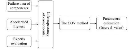
Figure 1: Parameters estimation of Weibull distribution based on the COV method

2 Fault Tree Analysis (FTA)

2.1 Model Construction of a Fault Tree

FTA is a logical and diagrammatic method for evaluating the failure probability of an accident. Fault tree includes various events, logic gates and other corresponding symbols.A significant failure or undesirable event is usually referred to as a top event since it appears at the top of the fault tree. Depending on the function of the logic gates, logic gates can be divided into static logic gates and dynamic logic gates. Static logic gates mainly include AND gate, OR gate and NOT gate while dynamic logic gates mainly include priority AND (PAND) gate, the function dependency (FDEP) gate, and spare (SP)gate, etc. Fault tree, including dynamic gates is a DFT, which extends static fault tree and can model the dynamic behaviors of system failure mechanisms, such as the function dependency events, spare gate, and the priorities. In the actual engineering, the first task is to construct the suitable fault tree model of the complex system. The construction of a fault tree usually requires a deep understanding of the system and its components. It usually includes the following steps: (1) Analyze the system configuration and fault mechanism and collect corresponding data derived from system design, operation data,and equipment technical specification. (2) Select and determine the top event. (3) Find the direct causes of the top event occurrence and connect the input events to the output events with the appropriate logic gates according to the logical relationship between these events. (4) Analyze each input event connected to the top event. If the event can also be further decomposed, we can define this event as the next level output event. (5) Repeat steps (2) to (4), and decompose step by step down until all input events can no longer be decomposed.

2.2 Parameters Estimation of Components Distributions

2.2.1 Parameters estimation for Exponential Distributions based on Fuzzy Sets Theory

In the practical engineering, the exponential distribution is applied widely in the reliability analysis, especially in the electronic equipment reliability assessment. The exponential distribution is a simple distribution with only one parameter. For a component whose lifetime follows an exponential distribution, the distribution function is F(t) =1 − e xp ( − λt), where λ is a distribution parameter. For fast technology innovation, the performance of complex systems such as reliability and stability has been greatly improved with the wide application of high technology on one hand, but on the other hand, the complexity of technology and structure increasing significantly raise challenges in system reliability evaluation and maintenance. Furthermore, high reliability of the systems causes the lack of sufficient fault data and epistemic uncertainty. So it is difficult to estimate precisely the failure rates of the basic events, especially for complex systems.In the paper, a hybrid method combined with expert elicitation through questionnaires and fuzzy sets theory is used to estimate the failure rates of the components which follow the exponential distribution [Duan, Zhou, Fan (2015)].

2.2.2 Parameters Estimation for Weibull Distributions based on the COV Method

The failure rate of a component with an exponential distribution is constant, which is usually not the case, and it will change over time. Weibull distribution first introduced by Waloddi Weibull in 1951, is widely used in reliability engineering and elsewhere due to its versatility and relative simplicity. For two-parameter Weibull distribution F(t,β,η),the distribution function is

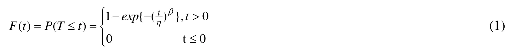
where η is the scale parameter and β is the shape parameter.

It has two parameters: shape parameter β and scale parameter η. The shape parameter, is also known as the Weibull slope. This is because the value of β is equal to the slope of the line in a probability plot. Different values of the shape parameter can have marked effects on the behaviour of the distribution. A change in the scale parameter has the same effect on the distribution as a change of the abscissa scale. In the practice engineering, it is a formidable task to assess two parameters of Weibull distribution at the same time using expert elicitation and fuzzy sets theory. Vast use of the COV method in engineering shows that it is easy for engineering applications. When the reliable lifetime of system components is available, the COV method can be employed to assess the parameters of their lifetime distributions [Mi, Li, Yang (2016)]. Fig. 1 shows the parameters estimation of Weibull distribution based on the COV method.

To meet the above challenge (3), we can get an approximate range of components’lifetime by incorporating the accelerated life test data, field failure data and experts evaluation. Accordingly, the lifetime of a component can be expressed as a bounded interval variable TY, and

where TLand TUare the lower and upper bounds of component lifetime respectively.Then the standard deviation of lifetime variable can be represented as

The mean value of Weibull distribution is E(T ) = ηΓ ( 1+1/β)and variance is Var(T) = η2[ Γ(1 + 2 /β) − Γ2(1+1/β)][Chen, Fang (2012); Mi, Li, Yang (2016)]. The coefficient of variation of Weibull distribution is

For Weibull distribution, the reliable lifetime tR, which is the lifetime of a system when system reliability equals to R, is given by

When the reliable lifetime tRand the lifetime variable TYare known, the parameters of Weibull distribution can be calculated by Eq. (2)-(5).

3 D-S theory and DEN

3.1 D-S theory

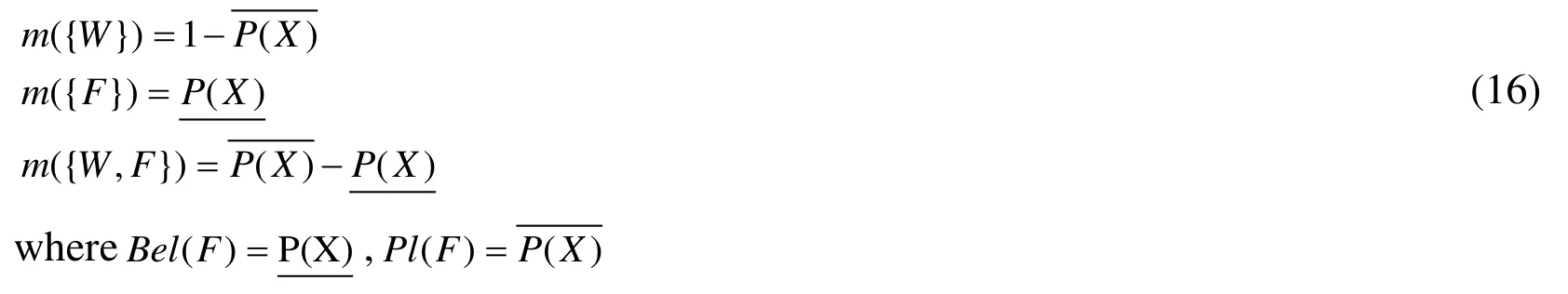
D-S theory is a theory of uncertainty that was first developed by Dempster [Dempster(1967)] and extended by Shafer [Shafer (1976)]. The idea of using D-S theory in reliability analysis was introduced by Dempster and Kong [Dempster, Kong (1988)]. D-S theory, a less restricted extension of probability theory is usually used to deal with epistemic uncertainty. The frame of discernment Θ is the set of all hypotheses for which the information sources can provide evidence. A basic probability assignment (BBA) on a frame of discernment Θ is a function mΘ:2Θ→[0,1]which maps beliefs masses on subsets of events as follows:

The two important measures of uncertainty provided by D-S theory are called belief and plausibility functions. They are defined by:

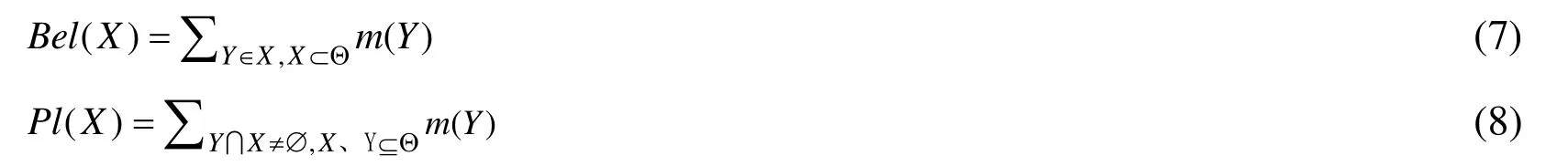
Belief function implies the summation of the possibility of all the subsets of hypotheses Y,which means the total trust of hypotheses Y. Plausibility function implies the level of suspicion. The interval [Bel(X), Pl(X)] represents the uncertainty of X. According to the above analysis, for X⊆Θ, there are following results:

3.2 DEN

Evidential Network (EN) based on graph theory and D-S theory. It is a promising graphical tool for representing and managing uncertainty [Helton, Johnson, Oberkampf,Sallaberry (2006)]. It is composed of nodes and directed arcs, in which nodes represent variables, directed arcs represent logical relationships between the nodes. EN model is represented by G = ((N, A), M), where (N, A) represents the graph, N={N1,···,Nl} is a set of nodes, A is a set of node’s arcs and M represents the belief distribution dependent relationship between the variables. DEN is based on a static EN and a temporal dimension [Philippe, Christophe (2008)]. It includes the initial network and the temporal transition network. Each time slice corresponds to a static evidence network, and the time slices are made up of a directed acyclic graph GT=＜ VT, ET＞and the corresponding conditional probabilities. The VTand ETare respectively nodes of time T and directed arcs. A directed arc links two variables belonging to different time slices andis used to denote the temporal transition network of time slices. Thencan be determined by

where T0is the initial network.

In the DEN, the present state of the time slice T only depends on the present state and the previous state,

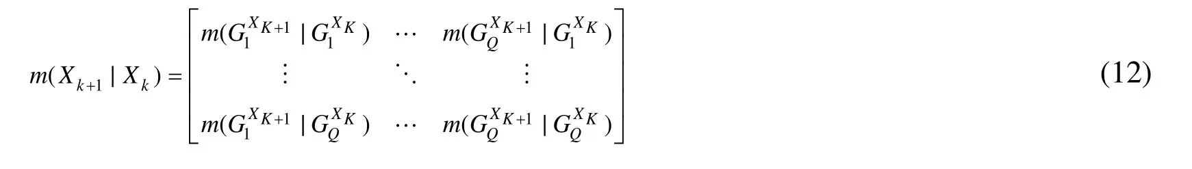
With this model, we define these impacts as transition-belief masses between the focal elements of the variable at time step k and those at time step k+1 and the conditional mass distribution tables (CMT) relative to inter-time slices is defined in Eq.12.

3.3 Mapping a DFT into a DEN

3.3.1 System Reliability Model of Evidential Network

In our evidence theory [Curcurù, Galante, La, (2012)],Θ={Wi, Fi}is the knowledge framework of a component i and the focal elements are given by

where {Wi},{Fi}and { Wi,Fi}denote respectively the working, the failure state and the epistemic uncertainty state of the component i.

The interval [B el(Wi) Pl(Wi)]represents the interval probability of the component i is in working state at time t, i.e.Bel(Wi)is the lower probability of the component i in the working state and Pl(Wi)is the corresponding upper probability. Moreover,Pl(Wi) − Bel(Wi)is represented as the epistemic uncertainty. Then the BPAs about component i is computed as:

When the component i follows the exponential distribution and the interval failure rateof the component is known, the bounds of the component reliability at a mission time T can be calculated by:

When the component j obeys to the two-paramYeters Weibull distribution, and the reliable lifetime tRtogether with the lifetime variable T are known, the bounds of the component reliability can be computed by Eq.(1)-(5).

So the upper and lower bounds of the component reliabilityare equivalent to the BPA in the DEN:

3.3.2 Mapping Static Logic Gates into DEN

When all the input components Xi(i=1,…, n) of an AND gate fail, the output of the gate fails. The conditional probabilities of each node in the static evidential network have been discussed in detail in [Philippe, Christophe (2008)]. Fig. 2 shows an AND gate and its equivalent DEN. Tab. 1 and 2 give the CMT of node A (T+ΔT) and node E (T+ΔT)respectively.

Figure 2: An AND gate and its equivalent DEN

Table 1: The CMT of node A (T+ΔT)

Table 2: The CMT of node E (T+ΔT)

3.3.3 Mapping Dynamic Logic Gates into DEN

DFT extended the traditional fault tree by defining some dynamic gates to capture the sequential and functional dependencies. Usually, there are six types of dynamic gates defined: the Functional Dependency Gates (FDEP), the Cold Spare Gates (CSP), the Hot Spare Gates (HSP), the Warm Spare Gates (WSP), the Priority AND Gates (PAND), and the Sequence Enforcing Gates (SEQ). The following section briefly discusses a CSP gate as it is used later in the example. The CSP gate includes one primary input and one or more alternate inputs. When the primary fails, the alternate inputs can be used instead of the primary input, and in turn, when this alternate input fails, it is replaced by the next alternate input, and so on until the CSP spare fails. Fig. 3 shows a CSP gate and its equivalent DEN. Tab. 3 shows the CMT of the node B(T+ΔT) and the CMT of output node E(T+ΔT) is shown in Tab. 4.

Figure 3: A CSP gate and its equivalent DEN

Table 3: The CMT of the node B (T+ΔT)

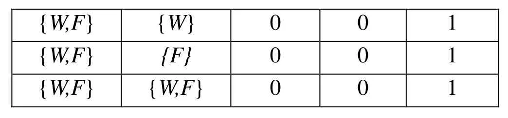
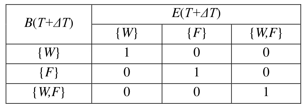
Table 4: The CMT of the node E (T+ΔT)

4 Calculating Reliability Parameters

4.1 Calculating Reliability Parameters

After a DFT model is built, The DFT is converted into an equivalent DEN using the proposed method. Once the structure of the DEN is known and the probability tables are filled, the reliability parameters of the system can be calculated using the DEN inference algorithm. These reliability parameters mainly include system unreliability, DIF and BIM,which can be used for fault diagnosis and system optimization design.

4.1.1 Calculating Reliability Parameters System Unreliability

Calculating the system unreliability is very simple using the following equation:

4.1.2 DIF

DIF is defined conceptually as the probability that an event has occurred given that the top event has also occurred. DIF is the cornerstone of reliability based diagnosis methodology. DIF can be used to locate the faulty components in order to minimize the system checks and diagnostic cost. It is given by:

where i is a component in the system S;P(i|S )is the probability that the basic event i has occurred given the top event has occurred.

Suppose the system has failed at the mission time. We input the evidence that system has failed into DEN and get the DIF of components using the inference algorithm.

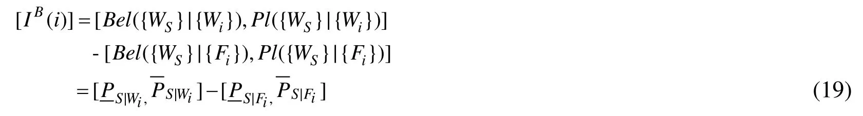
4.1.3 BIM

Birnbaum first introduced the concept of a components’ reliability importance in 1969.This measure was defined as the probability that a component is critical to system failures,i.e. when component i fails it causes the system to move from a working to a failed state.BIM of a component i can be interpreted as the rate at which the system’s reliability improves as the reliability of component i is improved [Mohamed, Walter, Felipe (2013)].Analytically, Birnbaum’s importance interval measure of a component i can be defined using D-S theory by the following equation.

4.2 Importance Sorting Method based on the Possibility Degree

DFT describes the logic relationships of system failure events and expresses the system structure. On the basis of the proposed assessment method, we can obtain interval values of system reliability and the importance of each component. The importance of components is related to the system structure, the lifetime distribution of each component and the mission time. Therefore, the ranking of component importance will be significant for improving the system design and determining the detection site of system when it is failed. It also can give the guidance for developing a checklist for system diagnosis.However, these interval values are not sufficient to rank components. To do this, we have to convert these interval values to a probability measure. Such a transformation is called a probabilistic transformation. The most known probabilistic transformation is the pignistic transformation BetP. It was introduced by Smets and Kennes [Smets, Kennes (1994)] and corresponds to the generalized insufficient reason principle: a BPA assigned to the union of n atomic sets is split equally among these n sets. It is defined for any set B ⊆ Xand B≠∅by the following:

where | A |denotes the cardinality of A ⊆ X. We should note that in the case of binary systems and closed word hypothesis (i.e.m(∅) = 0), the pignistic system reliability BetRSis given by:

In this paper, a sorting method based on the possibility degree is used to rank the importance of components represented by interval numbers [Moore, Lodwiek (2003); Li,Gu (2008)]. An interval number can be expressed as, whereand. For interval numbersand, the length of the interval numbers, lab is given by

If lab=∅, the intersection of interval number a and interval number b is empty. Then the possibility of a>b can be defined as

When there is any set of interval numbersi= 1,2,...,n, then by pairwise comparison of the interval numbers using the Eq. (22) and (23), the corresponding possibility pij= p(a ＞b)can be obtained and a possibility matrix P =is built.Then denoteas the row sum of the possibility matrixas the corresponding row sum vector. The interval numberwill be sorted based on possibility degree of vector λi. This method can be used to assess and compare the importance of each component with respect to the system. When comparing the possibility degree based ranking method with the deterministic sorting method base on the pignistic transformation, the distinct advantage of the possibility degree based method is that it not only helps for ranking the interval numbers, but also gives an estimation of the difference degree of two interval numbers. In addition, it can reflect the uncertainty of interval numbers. Therefore, this method is much more adaptive to engineering practice and has great theoretical significance.

5 A numerical Example

An illustrative example is given to illustrate how the proposed method can be used to perform the reliability analysis for the braking system using DFT and DEN. Suppose all components follow the exponential distribution or two-parameter Weibull distribution.For the components with an exponential distribution, the interval failure rates of the basic events for the braking system can be calculated using the expert elicitation and the fuzzy sets theory. For the components with a two-parameter Weibull distribution, the interval failure rates are calculated using the COV method. Fig. 4 shows a DFT for service braking failure of braking system. The interval failure rates of basic events are shown in Tab. 5.

In this numerical example, component X2 is assumed to follow the Weibull distribution and other components follow the exponential failure distribution. The interval lifetime[tR=0.95, tR=0.5]of X2 is [2100, 4200] using the general accelerated life test and the parameters are obtained as follows: β=3.304, η=[4692.7, 5159.7]. For quantitative analysis, we map the DFT into the equivalent DEN. Supposing that the mission time is T=2000 hours and ΔT=500 hours, the BPA of each root node and the conditional probability tables of each intermediate node can be calculated according to Section 3.3.

Unreliability of the braking system can be obtained. Tab. 6 shows the top event occurrence probabilities at the different mission time. Tab. 7 gives the DIF and BIM of components for the braking system respectively. The obtained importance measures are interval values because in the presence of epistemic uncertainty the belief measures are not equal to the plausibility measures. However, within these interval values of importance measures, it is very difficult to rank components’ importance. A sorting method based on the possibility degree is used to rank the DIF of components. According to the sorting method of interval numbers in Section 4.2, the possibility matrices P can be calculated by Eq. (23). Then the ranking vectors λiof matrices P can be computed as

λ=(20.5, 17.5, 6.835, 2.5, 15.6, 9.14, 14.02, 12.49, 6.622, 6.622, 1.027, 13.37, 10.53,5.366, 0.9732, 5.458, 5.458, 23.48, 23.48, 19.00, 14.24, 23.48, 23.48, 19.00, 14.24,23.596).

Figure 4: A DFT for service braking failure of braking system

According to ranking vectors λi, from the most critical component to the lesser one, the ranking result of the components importance DIF can be represented as

X26>X18(X19) >X22(X23) >X1>X20(X24)>X2>X5>X21(X25)

> X7>X12>X8>X13>X6>X3>X9>X10>X16>X17>X14>X4> X11>X15

where the symbol “>” is denoted as the optimal order relation of two interval numbers.The related interval values of DIF can also be converted into crisp values in order to rank components by means of the pignistic transformation and the ranking is

X26>X18(X19) >X22(X23) >X1>X20(X24)>X2>X5>X21(X25)> X7>X12

> X13>X6>X3>X9>X10> X16 >X17>X14>X4>X15>X8>X11

Obviously, the ranking based on the possibility degree is a little different from the one by means of the pignistic transformation and the former is more reasonable because the latter neglects the difference degree of two interval numbers. From the ranking results based on the possibility degree, we can see that the DIF of X15 stays at a low level. This is because X15 is a cold spare gate, which can only be active when the primary input fails.Additionally, DIF measure indicates that the component X26 is the most critical in the system from a diagnosis perspective, and it should be first diagnosed to fix the braking system when the system fails. If we have the potential to upgrade components, the component X26 is the most important in the system and improving its reliability will have more influence on the system reliability.

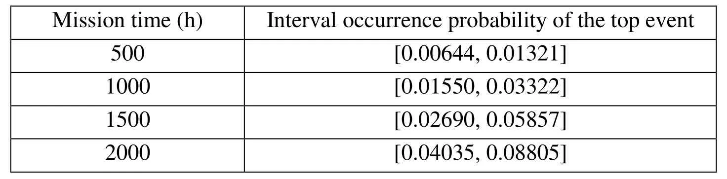
Table 6: The interval failure rates of system components

Table 7: The DIF and BIM of components for the braking system

6 Conclusions

In this paper, we have discussed the use of DFT and DEN to evaluate complex systems reliability under epistemic uncertainty. Specifically, it has emphasized three important issues that arise in engineering diagnostic applications, namely the challenges of failure dependency, different life distributions and epistemic uncertainty. In terms of the challenge of failure dependency, DFT is used to model the dynamic behaviours of system failure mechanisms. In terms of the challenge of multiple life distributions, a mixed life distribution is used to analyse complex systems; In terms of the challenge of epistemic uncertainty, the failure rates of the basic events for complex systems are expressed in interval numbers. For a component whose lifetime follows an exponential distribution, a hybrid method combined with expert elicitation and fuzzy sets is used to estimate the failure rate of the component. For a component whose lifetime follows a Weibull distribution, the COV method is employed to assess the parameters of the lifetime distributions. Furthermore, we calculate some reliability results by mapping a DFT into an equivalent DEN in order to avoid some disadvantages. In addition, a sorting method based on the possibility degree is proposed to rank the importance of components represented by interval numbers in order to obtain the most critical components, which can be used to provide the guidance for system design, maintenance planning and fault diagnosis. Finally, a numerical example is provided to illustrate the availability and efficiency of the proposed method.

Acknowledgement This work was supported by the National Natural Science Foundation of China (71461021), the Natural Science Foundation of Jiangxi Province(20151BAB207044), the China Postdoctoral Science Foundation (2015M580568) and the Postdoctoral Science Foundation of Jiangxi Province (2014KY36).

Lisnianski, A. (2007): Extended block diagram method for a multi-state system reliability assessment. Reliability Engineering & System Safety, vol.92, no.12, pp. 1601-1607.

Rahman, F. A.;Varuttamaseni, A.; Kintner-Meyer, M. (2013): Application of fault tree analysis for customer reliability assessment of a distribution power system.Reliability Engineering & System Safety, vol. 111, pp. 76-85.

Shrestha, A.; Xing, L. (2008): A logarithmic binary decision diagram-based method for multistate system analysis. IEEE Transactions on Reliability, vol. 57, no. 4, pp. 595-606.Yevkin, O. (2005): An Efficient Approximate Markov Chain Method in Dynamic Fault Tree Analysis. IEEE Transactions on Reliability, vol.32, pp. 1509-1520.

Chen, Y.; Zheng, Y.; Luo, F. (2016): Reliability evaluation of distribution systems with mobile energy storage systems. IET Renewable Power Generation, vol.10, no.10, pp.1562-1569

Kabir, S.; Walker, M.; Papadopoulos, Y. (2014): Reliability analysis of dynamic systems by translating temporal fault trees into Bayesian networks. Model-Based Safety and Assessment, Springer International Publishing, pp. 96-109.

Dugan, J. B,; Bavuso, S. J,; Boyd, M. A. (1992): Dynamic fault-tree models for faulttolerant computer systems. IEEE Transactions on Reliability, vol. 41, pp. 363-377.

Wu, X.; Liu, H.; Zhang, L. (2015): A dynamic Bayesian network based approach to safety decision support in tunnel construction. Reliability Engineering & System Safety,vol. 134, pp. 157-168.

Khakzad, N. (2015): Application of dynamic Bayesian network to risk analysis of domino effects in chemical infrastructures. Reliability Engineering & System Safety, vol.138, pp. 263-272.

Kabir, S.; Walker, M.; Papadopoulos, Y. (2016): Fuzzy temporal fault tree analysis of dynamic systems. International Journal of Approximate Reasoning, vol.77, pp. 20-37.

Ge, D.; Lin, M.; Yang, Y. (2015): Quantitative analysis of dynamic fault trees using improved Sequential Binary Decision Diagrams. Reliability Engineering & System Safety,vol. 142, pp. 289-299.

Merle, G.; Roussel, J. M.; Lesage, J. J. (2015): Probabilistic algebraic analysis of fault trees with priority dynamic gates and repeated events. IEEE Transactions on Reliability,vol. 134, no. 1, pp. 250-261.

Chiacchio, F.; Cacioppo, M.; D'Urso, D. (2013): A Weibull-based compositional approach for hierarchical dynamic fault trees. Reliability Engineering & System Safety,vol. 109, pp. 45-52.

Mahmood, Y. A.; Ahmadi, A.; Verma, A. K. (2013): Fuzzy fault tree analysis: A review of concept and application. International Journal of System Assurance Engineering and Management, vol. 4, no. 1, pp. 19-32.

Mhalla, A.; Collart D S.; Craye, E. (2014): Estimation of failure probability of milk manufacturing unit by fuzzy fault tree analysis. Journal of Intelligent and Fuzzy Systems,vol. 26, no. 2, pp. 741-750.

Kabir, S.; Walker, M.; Papadopoulos, Y. (2016): Fuzzy temporal fault tree analysis of dynamic systems. International Journal of Approximate Reasoning, vol. 77, pp. 20-37.

Li, Y. F.; Huang, H. Z.; Liu, Y. (2012): A new fault tree analysis method: Fuzzy dynamic fault tree analysis. Eksploatacja i Niezawodnosc - Maintenance and Reliability,vol. 14, no. 3, pp. 208-214.

Li, Y. F.; Mi, J.; Liu, Y. (2015): Dynamic fault tree analysis based on continuous-time Bayesian networks under fuzzy numbers. Proceedings of the Institution of Mechanical Engineers, Part O: Journal of Risk and Reliability, vol. 229, no. 6, pp. 530-541.

Mi, J.; Li, Y. F.; Yang, Y. J. (2016): Reliability assessment of complex electromechanical systems under epistemic uncertainty. Reliability Engineering & System Safety, vol. 152, pp. 1-15.

Duan, R.; Zhou, H.; Fan, J. (2015): Diagnosis strategy for complex systems based on reliability analysis and MADM under epistemic uncertainty. Eksploatacja i Niezawodnosc – Maintenance and Reliability, vol. 17, no. 3, pp. 345–354.

Chen, J. D.; Fang, X. Z. (2012): The reliability evaluation in the case of Weibull or lognormal distributions. Jouranl of Application Statistics and Management, vol. 31, no. 5,pp. 835-848.

Dempster, A. P. (1967): Upper and lower probabilities induced by a multivalued mapping. Annals of Mathematical Statistics, vol. 38, pp. 325–339.

Shafer, G. (1976): A Mathematical Theory of Evidence. Princeton University Press.

Dempster, A.; Kong, A. (1988): Uncertain evidence and artificial analysis. Journal of Statistical Planning and Inference, vol. 20, pp. 355-368.

Helton, J. C.; Johnson, J. D., Oberkampf, W. L.; Sallaberry, C. J. (2006): Sensitivity analysis in conjunction with evidence theory representations of epistemic uncertainty.Reliability Engineering & System Safety, vol. 91, no. 10, pp. 1414-1434.

Philippe, W.; Christophe, S. (2008): Dynamic evidential networks in system reliability analysis: A Dempster-Shafer Approach. Proceedings of the 16th Mediterranean Conference on Control & Automation, Ajaccio-Corsica, France. June 25-27, pp. 603-608.

Curcurù, G.; Galante, G. M.; La, F. C. M. (2012): Epistemic uncertainty in fault tree analysis approached by the evidence theory. Journal of Loss Prevention in the Process Industries, vol. 25, no. 4, pp. 667-676.

Mohamed, S.; Walter, S.; Felipe, A. (2013): Extended component importance measures considering aleatory and epistemic uncertainties. IEEE Transactions on Reliability, vol.62, no. 1, pp. 49-65.

Smets, P.; Kennes, R. (1994): The Transferable Belief Model. Artificial Intelligence, vol.66, pp. 191–243.

Moore, R.; Lodwiek, W. (2003) Interval analysis and fuzzy set theory. Fuzzy and System, vol. 135, no. 1, pp. 5-9.

Li, D. Q.; Gu, Y. D. (2008): Method for ranking interval numbers based on possibility degree. Journal System Engineering, vol. 23, no. 2, pp. 243–246.