Assessment of the predictive capability of RANS models in simulating meandering open channel flows*
2017-03-09JianyinZhou周建银XuejunShao邵学军HongWang王虹DongdongJia假冬冬
Jian-yin Zhou (周建银), Xue-jun Shao (邵学军), Hong Wang (王虹), Dong-dong Jia (假冬冬)
1.Key Laboratory of River Regulation and Flood Control of MWR, Changjiang River Scientific Research Institute, Wuhan 430010, China
2.State Key Laboratory of Hydroscience and Engineering, Tsinghua University, Beijing 100084, China, E-mail: zhoujianyin57@163.com
3.State Key Laboratory of Hydrology-Water Resources and Hydraulic Engineering, Nanjing Hydraulic Research Institute, Nanjing 210029, China
(Received August 5, 2015, Revised August 24, 2015)
Assessment of the predictive capability of RANS models in simulating meandering open channel flows*
Jian-yin Zhou (周建银)1,2, Xue-jun Shao (邵学军)2, Hong Wang (王虹)2, Dong-dong Jia (假冬冬)3
1.Key Laboratory of River Regulation and Flood Control of MWR, Changjiang River Scientific Research Institute, Wuhan 430010, China
2.State Key Laboratory of Hydroscience and Engineering, Tsinghua University, Beijing 100084, China, E-mail: zhoujianyin57@163.com
3.State Key Laboratory of Hydrology-Water Resources and Hydraulic Engineering, Nanjing Hydraulic Research Institute, Nanjing 210029, China
(Received August 5, 2015, Revised August 24, 2015)
The predictive capability of Reynolds-averaged numerical simulation (RANS) models is investigated by simulating the flow in meandering open channel flumes and comparing the obtained results with the measured data. The flow structures of the two experiments are much different in order to get better insights. Two eddy viscosity turbulence models and different wall treatment methods are tested. Comparisons show that no essential difference exists among the predictions. The difference of turbulence models has a limited effect, and the near wall refinement improves the predictions slightly. Results show that, while the longitudinal velocities are generally well predicted, the predictive capability of the secondary flow is largely determined by the complexity of the flow structure. In Case 1 of a simple flow structure, the secondary flow velocity is reasonably predicted. In Case 2, consisting of sharp curved consecutive reverse bends, the flow structure becomes complex after the first bend, and the complex flow structure leads to the poor prediction of the secondary flow. The analysis shows that the high level of turbulence anisotropy is related with the boundary layer separation, but not with the flow structure complexity in the central area which definitely causes the poor prediction of RANS models. The turbulence model modifications and the wall treatment methods barely improve the predictive capability of RANS models in simulating complex flow structures.
RANS model, secondary flows, boundary layer separation, turbulence model, meandering channel, near-wall treatment
Introduction
During recent years, three-dimensional numerical models were widely used in simulating flows and sediment transports in both laboratory flumes and natural rivers. In current models for flows in open channelsand rivers, the unsteady three-dimensional Navier-Stokes equations are not directly solved, because it is computationally expensive carrying out direct numerical simulations (DNS) for real water flows at high Reynolds numbers. Instead, Reynolds-averaged Navier-Stokes equations are considered in most models because of their computational expedience and sufficient accuracy. To solve Reynolds-averaged Navier-Stokes equations, a Reynolds-averaged numerical simulation (RANS) turbulence model is required to model the Reynolds stress tensor. If the Boussinesq approximation is used to model the Reynolds stress tensor, the turbulence model is an isotropic eddy viscosity model, otherwise it is non-isotropic. Correspondingly, a RANS model which employs an isotropic turbulence models is often referred to as an isotropic RANS model, otherwise it is called a non-isotropic RANS model. Though there are many non-isotropicRANS turbulence models[1], few of them have wide verifications and applications. Several isotropic RANS turbulence models, including the SA model, thek-εmodel, thek-ωmodel and the SST model, play a dominant role in practical applications. Such models were applied to predict flows in curved open channel flumes[2,3], and flows in natural rivers[4,5]and to model delta morpho-dynamics[6]. Despite these extensive applications, the capability of the RANS models in predicting complex flow structures remains to be investigated.
Previous studies show that the RANS models can capture the curvature-driven secondary flow within a bend, while they may encounter difficulty in predicting other key features such as the shear-stress derived outer-bank cell(OBC)[7,8]and the boundary shear layers[9]. The OBC is a small circulation near the outer-bank and the water surface, which rotates in the opposite direction with the main circulation caused by the channel curvature. The boundary shear layer refers to a district attached to the boundary, which is separated from the central flow as a result of the boundary layer separation. These features affect the flow structure and the bed shear stresses, and are thought to play an important role in the sediment transport and the river evolution[9]. Some studies compared the performance of the RANS models and the LES for predicting flows in curved channels[7,9,10,11]. While the flow fields predicted by the RANS and LES models agree well as shown in Ref.[11], discrepancies do exist in other tests. The disagreement is commonly attributed to the turbulence anisotropy. Kang and Sotiropoulos[9]assessed the predictive capabilities of the isotropic RANS model in a natural-like meandering channel by comparing with measured data and LES predictions. Comparisons show that the flow features in regions of high level of turbulence anisotropy are not well predicted by the RANS model. On the other hand, the local turbulence anisotropy level is a function of geometric and flow conditions. It is concluded that application of isotropic RANS models to simulate the turbulent flow in meandering channels might lead to nonphysical results without full understanding of the inherent limitations of such models.
Inaccurate predictions of the RANS models were found in many cases, some issues remain to be solved, including the influencing factors, the inherent causes and the extent of inaccuracy under different circumstances.
Despite various disadvantages, RANS models generally well simulate the primary flow structure, as was demonstrated in previous studies. The good performance may be probably due to the fact that the flow structures in those test cases are relatively simple, with only one primary circulation in each cross section. The suggestion is supported by the fact that despite the inaccurate prediction of some features, the longitudinal velocities simulated by RANS models are at least not significantly worse than those obtained by the LES and are well consistent with measured data. However, the flow structure might be much more complex in practical cases due to the possible complicated topographic configurations, hydraulic structures and flow conditions. One is not convinced about the capability of the RANS models in simulating complex flows where two or more significant circulations exist, interact with and dominate the flow structures. In view of the wide applications of the RANS models, further investigation is necessary. In addition, the relation between the turbulence anisotropy and the performance of a RANS model is an interesting topic. Experientially, it would be expected that some hydraulic and numerical factors such as the turbulence anisotropy level, the flow structure complexity, the turbulence models and the near wall treatment would affect the performance of RANS models.
To test the performance of RANS models in predicting complex flow structures, detailed information is necessary. Many experiments were conducted to provide quantitative descriptions and detailed information of the bend flow[2,12,13]. But not all of them are suitable to be used to test the predictive capability of RANS models. To demonstrate the predictive capability of RANS models, some features related to the Reynolds shear stress should be considered, for example, the OBC. These features are usually seen in a bend with a high ratio, of the central line radius to the channel width, i.e.,R/B. Few experiments were carried out in a sharp bend(R/B<2.5-3.0)[14]. Most flumes in experiments contain only one bend, so that the secondary flow structure is relatively simple, e.g., with a dominant curvature-induced circulation along with a small OBC. By contrast, natural meandering rivers often consist of several reverse bends. Reverse bends give rise to adverse secondary flows that may lead to complex flow structures. Some experiments of consecutive reverse bends were carried out[10,15,16]. However, bends in those experiments are weakly or mildly curved, and adjacent bends are connected by straight transitional sections. The connecting section reduces the effect of an upper bend on the flow structure in its followed bend to such extent that each bend performs as a single bend in simple flow structures. Recently, He[17]conducted a laboratory flume experiment containing several consecutive reverse sharp bends. In this experiment, consecutive sharp bends are connected directly, in other words, without transitional sections between adjacent bends. Besides, the water depth-width ratio is 1/4, which enhances the complexity of the three-dimensional flow structure. The configuration and the flow condition of this experiment provide very complex flow structures and also a pre-cious case for bend flow researches and numerical model tests.
Our objective is to investigate the predictive capability of RANS models for bend flows with complex structures. To examine the effects of different turbulence models and boundary conditions, two types of widely used RANS turbulence models are considered. Various turbulence model modifications and different near wall treatments are tested as well. Among various experiments, those of Chang[15]and He[17]are chosen as test cases because of their different configurations, flow conditions and above all the flow structure complexity. Simulating results are compared with measured data and the performances are analyzed to shed new light on the predictive capability and the limitation of RANS models.
1. Numerical model
The original code of the present RANS model is the same as that used in Jia et al.[5], and various turbulence models were coded by the present author. Two types of turbulence models are used in this work: (1) thek-εturbulence models, including the standard, RNG, Realizablek-εand a cubic nonlineark-εturbulence models developed by Craft[18](hereinafter referred to as SKE, RNG, RKE and NKE, respectively), (2) the shear stress transport (SST) turbulence models, including the standard version of Menter[19], the rotation/curvature correction version of Smirnov and Menter[20]and the simplified rotation/ curvature correction version of Hellsten[21]and Mani et al.[22](hereinafter referred to as SST, SST-RC, SSTRCH). The nonlineark-εmodel of Craft[18]is chosen because it is a cubic model which is essential to capture the flow curvature and has been used in many researches.

For the eddy viscosity turbulence model, the Reynolds stress is modeled by whereδijis the Kronecker delta,kis the turbulence kinetic energy,νtis the turbulence viscosity (eddy viscosity) andbijis the nonlinear part. Ifbijis equal to zero, the turbulence model is reduced to a linear model, otherwise it is a nonlinear model. A linear model is an isotropic model, while a nonlinear model may not be an isotropic model. The eddy viscosity turbulence model is used to solve the Reynolds stress tensor, that is, to solvek,νtandbij.
To simplify this presentation, the details of turbulence models are not included.
The codes are based on curvilinear grids with a collocated grid system. The turbulent kinetic energyk, its dissipation rateεand the specific dissipation

2. Test cases and comparisons
In order to make comparisons, we choose two cases of consecutive open channel bends. Case 1 contains a straight connecting section between adjacent bends, while no connecting section exists in Case 2. The scales of the two cases are summarized in Table 1,and the configurations are illustrated in Figs.1 and 2. The flow structure in Case 1 is typical for flows in a bend, consisting of a curvature driven circulation with a tiny OBC in few sections after the bend apex. Case 2 is given a particular attention because of its complex flow structures.

Table 1 Scales of the two experiments

Fig.1 Configuration and dimension of Case 1[15](m)
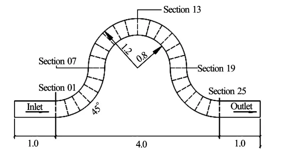
Fig.2 Configuration and dimension of Case 2[17](m)
2.1Case 1: Mildly curved bends with a straight connecting section
The experiment was carried out by Chang[15]. The water depthhis 0.115 m, and the bulk velocityUis 0.366 m/s. The channel has rectangular cross sections and its bed and sidewalls are smooth. Numerical simulations with the above mentioned two types of turbulence models are performed with exactly the same grids. After trail computations, the selected grid dimensions are 261×31×11 (downstream×transverse× vertical), with grid refinement near surrounding boundaries while keeping the wall distance in a suitable range for the standard wall function.
Comparisons of the longitudinal and lateral velocity profiles at Sections S0 and PI/8 are listed in Figs.3-4, where it is shown that the flow structure in the second bend does not differ from a typical flow structure in a single bend, suggesting that the influence of the previous bend is negligible. Numerical predictions of all turbulence models agree well with the experimental data. Among these models, RNG, RKE and NKE perform a little better than SKE in some locations, while SST-RC and SST-RCH do not show advantages over SST. No distinct difference exists among predictions of all models. However, just as inprevious researches[2,7,8], all models fail to predict the small outer-bank cell and its impact on the profile of the longitudinal velocity in both bends (y/b=0.064 in Section S0 andy/b=0.912in Section PI/8).

Fig.3 Comparison of longitudinal velocityUand lateral velocityVin Section S0

Fig.4 Comparison of longitudinal velocityUand lateral velocityVin Section PI/8
2.2Case 2: Sharply curved bends without connecting section
He[17]carried out the experiment in a laboratory curved open channel flume, which contains four 90ocurved sections that constitute three adjacent reverse bends. The cross shape of the flume is rectangular.
The flume is made of organic glass, and the bed and the sidewalls are hydraulically smooth. Twentyfive sections are marked through the entire curved channel in Fig.2 (from Section 01 to Section 25). For each section, the water levels at sidewalls and the central line are measured. Velocity data are obtained in all sections, except Section 01 and Section 12. This omission is insignificant for our purpose. The bed slope of the flume is 0.0003, and the flow rate is about 12.66 L/s. Water is recycled, and the flow rate is measured by a weir. The averaged depth of the outflow section is about 0.0953 m. The flow is kept steady during the experiment, and the bulk longitudinal velocity is 0.32 m/s.

Fig.5 Comparison of water surface level
To examine the effect of the wall treatment, two grid systems of different densities are used for numerical modeling. The dimension of the sparse grid system is 321×20×13 (downstream×transverse×vertical) nodes, while the dense grid system is 321×36×26 (downstream×transverse×vertical) nodes. Both grid systems are refined near the walls. The non-dimensional wall distances of the calculated grids next to the walls are 58 for the bed and 70 for the sidewalls insparse grids, both of which fit for the standard wall function method. In the dense grids, the corresponding values are 1.4 and 7.0, both are in the viscous sublayer.

Fig.6 (Color online) Comparison of typical secondary flow structures in each bend (The contour represents longitudinal velocity and the arrowed lines show the circulations. EX represents experiment)
Though all turbulence models are tested in modeling both cases, we will mainly compare results of RNG and SST models for simplicity. The results of the RNG and SST models are chosen because they perform best ink-εand SST type models, respectively and no essential difference exists among results of modeling with different turbulence models. Results of NKE model is also partially presented because it is a nonlinear turbulence model.
2.3Water surface slopes
Figure 5 compares the water surface level between experimental data and numerical predictions with sparse and dense grid systems. Although the trend of the water surface level through the whole channel is evident, the experimental data are quite fluctuated, which indicates the sampling error. Comparisons show that the computed water surface levels fit well with experimental data. Note that the range of the vertical coordinate starts not from zero. The averaged downstream slope of the water surface level is about 3.5% and the maximum transverse water surface slope is about 1%.
2.4Flow structure at typical sections
Figure 6 shows the comparison of the typical secondary flow structure in each bend under different modeling conditions. Generally, the flow structure becomes more complex downstream, and the prediction of the numerical model becomes worse. Experimentaldata indicate that, in the first bend (Section 04), similar to Case 1, a curvature induced circulation dominates the flow structure. In the lower bends, the flow structure becomes complex. For example, the secondary flow structure in Section 13, which is the middle section of the second bend, contains two circulations with about the same size and strength, but with opposite directions. This phenomenon has rarely been reported. The one near the surface and the right (inner) bank is the residual of the main circulation from the previous bend. Experimental data[17]illustrate that this circulation exists at least up to Section 15. This phenomenon implies that the residual motion of the secondary flow can sustain a much longer distance than the length of the first bend where it has been developed. As we could see, the flow structure in the second bend is more complex than in the first bend, and the complexity continues to enhance in the third bend (Section 23 in Fig.6). Therefore, the flow structure in a lower bend might be affected significantly by its upper bend or even the bend further upstream, which would lead to a complex flow structure. Results show that predictions of all models are similar. Comparisons indicate that numerical modelling reasonably simulates the secondary flow in the first bend but fails to simulate the secondary flow in the second and third bends. The deviation seems to accumulate downstream. Furthermore, it is indicated that numerical models properly predict the generation of most circulations but fail to simulate their evolution including the locations, the size and the strength.
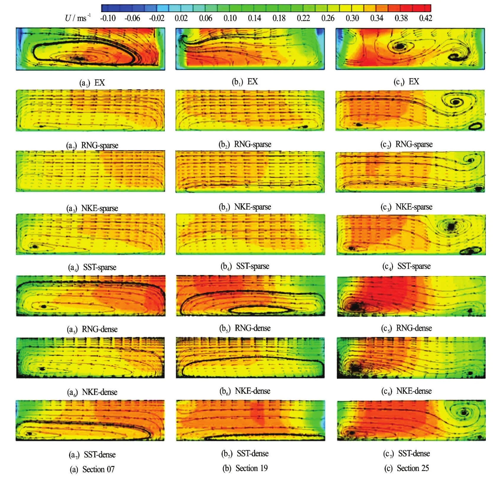
Fig.7 (Color online) Comparison of flow structure at transitional cross sections (The contour represents longitudinal velocity and the arrowed lines show the circulations. EX represents experiment)
Figure 7 compares the flow structure at transitional cross sections between adjacent bends and the exit section (Section 25) of the last bend. Experimental data show that the flow structures differ a lot in different sections, and no obvious trend of the flow structure evolution is observed. Especially, although located between the second and third bends, the flow structure in Sec tion 19 is r elatively s imple without obvious circulation.Fromthecomplexflowstructurebefore(Section 13) and after (Section 23) the location, we can infer that the adverse effect of the first, second and third bends leads to a weak circulation in Section 19. Comparisons show that, differences between predictions by using different turbulence models are not significant and numerical models perform better for Section 07 and Section 19 than for Section 25. Results also indicate that the longitudinal velocity distribution predicted by using a dense grid is a little better than that using a sparse grid.

Fig.8 Comparison of longitudinal velocity
2.5Detailed comparison of velocities
Figure 8 shows the comparison of vertical profiles of the longitudinal velocity in various sections under different modeling conditions. To keep things simple, only predictions of RNG and SST models are presented. Experimental data indicate that the longitudinal velocity profiles vary in different locations and are affected by the secondary flow because most of them do not follow a regular log profile. In general, numerical results agree well with experimental data, though discrepancy still exists in several sections. The results also show that modeling with dense grids generally performs better than that with sparse grids. These findings suggest that modeling with dense grids may simulate the secondary flow more accurately.
Figure 9 shows the comparison of the transverse velocity in the same sections as in Fig.8. The comparison reveals a trend that the performance of the numerical simulation becomes worse when the profiles become more irregular downstream. However, Section 19 is an exception. The prediction of Section 19 is better than those of Section 13 and its following sections. For the RNG model, comparisons show thatsimulations with dense grids generally perform better near the wall than those with sparse grids in some sections. The SST model performs a little better than the RNG model in the sparse grid system, while the RNG model performs a little better than the SST in the dense grid system. Generally, no essential difference exists among all predictions.
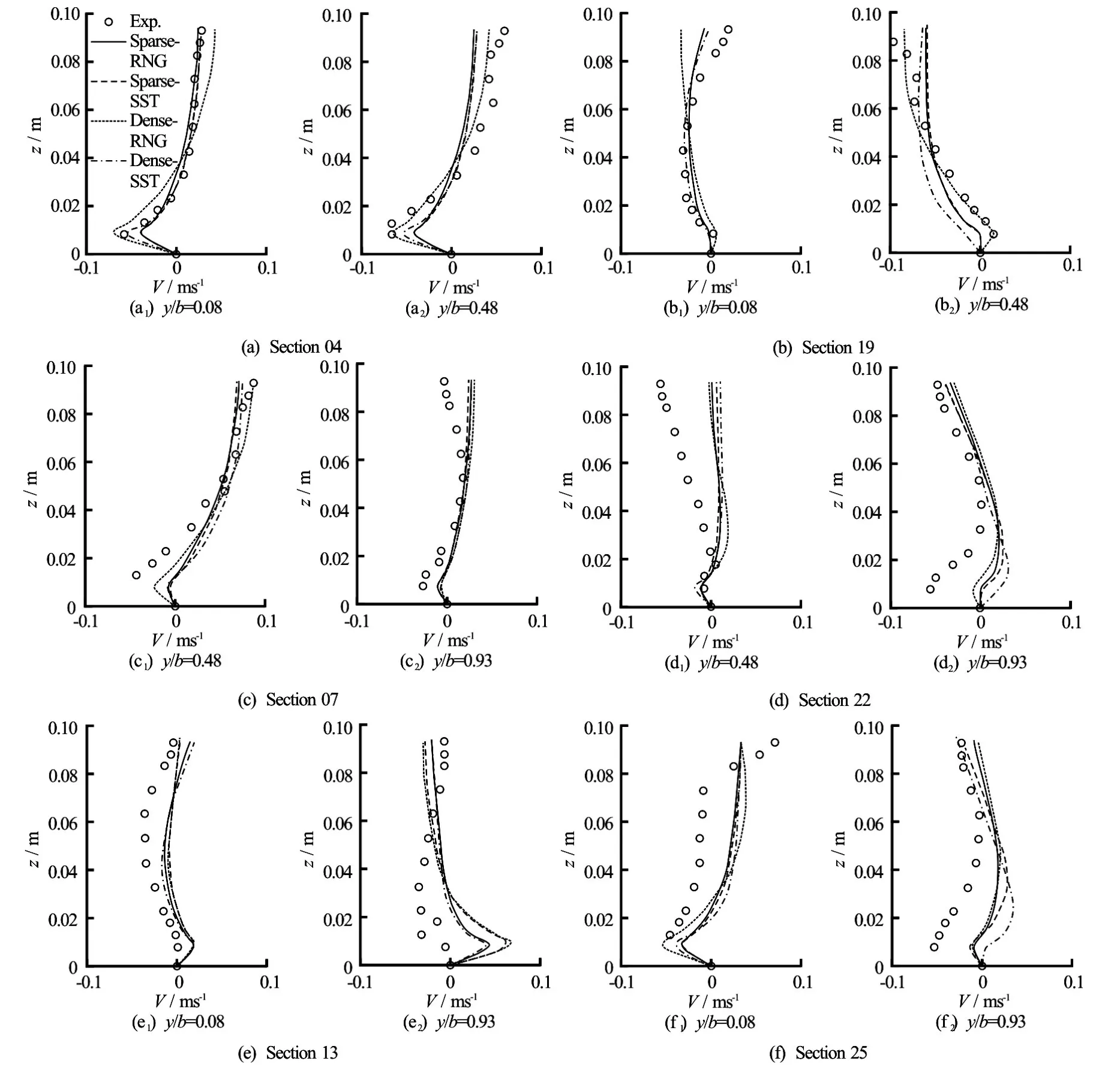
Fig.9 Comparison of lateral velocity evolving in the first bend
3. Discussions
3.1Location of poor performance
The comparisons in the previous section show that differences of turbulence models and grid densities are not essential for the capability of numerical models. The grid density applied in Case 1 is equivalent to the sparse grid in Case 2, since the near wall grid distances in both cases are suitable for the wall function. The numerical predictions of Case 1 fit quite well with the measured data. Thus further refinement is not applied in Case 1. In Case 2, two grid systems are applied. However, numerical predictions do not agree well with the measured data in many sections.
Comparisons show that, at locations where the longitudinal velocity profiles are irregular (such asy/b=0.08of Section 07 andy/b=0.08, 0.93 of Section 19 in Fig.8), the predictions are not as good as others. Those locations are all at corners of the water surface and the bank wall. By comparing the predictions with the experimental data, it is shown that the irregular regions are caused by small, local, vertical or longitudinal circulations in the form of shear layers (y/b=0.08of Section 07,y/b=0.93of Section 19 andy/b=0.08of Section 22 in Fig.8) and a secondary circulation (y/b=0.08of Section 19 in Fig.8),respectively. To demonstrate the causes, Fig.10 illustrates the experimental longitudinal velocity in Section 04 and Section 19, from which regions of negative longitudinal velocity are found. These regions are where the boundary layer separates from the central flow and the numerical models perform poorly.

Fig.10 Experimental longitudinal velocities
Similar features were revealed in Ref.[9], where the inner and outer bank shear layers also result from the separation of boundary layers. Not surprisingly, small local circulations appear in the present work and in Ref.[9] (Figs.3 and 4 in that paper), which challenges the ability of RANS models. Reference [9] further revealed that high turbulence anisotropy was found along the inner and outer bank shear layers, and considered it the main cause of the failure of the RANS model. To verify its finding, we also calculate the second invariant of the anisotropy as in Ref.[9], which is defined as follows:

wheredenotes velocity fluctuations in theith direction,δijis the Kronecker delta, and the overbar denotes the temporal (or Reynolds) averaging. Figure 11 illustrates the level of turbulence anisotropy in Section 04 and Section 19. The contours confirm the finding that the high level turbulence anisotropy is located where the boundary layer separation occurs.
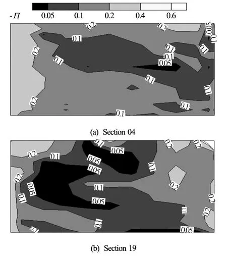
Fig.11 Level of turbulence anisotropy −Πof Case 2
3.2Flow structure and distribution of turbulence anisotropy
Previous comparison of Case 2 shows a trend that, while the water flows downstream, the flow structure generally tends to be more complex, meanwhile, the prediction of the secondary flow becomes worse. Following the explanation of the previous paragraph, we calculate the overall turbulence anisotropy at each section using the measured data. Figure 12 illustrates the distribution of the sectional averaged turbulence anisotropy along the flume and no evident tendency could be observed. Unexpectedly, the value of Section 19 is a peak instead of a trough. Therefore, the level of the section-averaged turbulence anisotropy could not explain or indicate the mentioned trend of the modelling performance or the better prediction in Section 19.

Fig.12 (Color online) Distribution of section-averaged turbulence anisotropy
Though Section 19 is located between the second bend and the third bend, the secondary flow structure in this section is relatively simple as the secondary flow direction is the same in most area of the section and circulations only exist at the corners. Meanwhile, the numerical prediction of the transverse velocity in Section 19 is better than in sections before and after it. On this basis, a more universal relation can be suggested, that is, the more complex the flow structure is, the worse the secondary flow prediction becomes. In the first bend, only one primary circulation exists, and the predictions agree well with the measured data. In the second and third bends, when two or more primary circulations exist, the secondary flow prediction becomes unreliable, and if the flow structure is simple, as in Section 19, the prediction would be much better.
Furthermore, it is found that in all sections, the high level of anisotropy is observed near the boundaries, while the turbulence anisotropy level remains low in the central area, not depending on the complexity of the flow structure. This phenomenon is consistent with the boundary layer theory and the turbulence features in Ref.[9]. It indicates that the anisotropy is closely related to the boundary layer where a strong shear stress exists. Meanwhile, the complex flow structures stem from the boundary layer because new circulations are firstly generated from the wall boundary. This is convinced by the measured data of Case 2. Due to the effect of reverse bends, some new circulations grow up, interactive with and even replacing previous primary circulations. These processes take a long distance and make the flow structures in the central area complex. Actually, as mentioned above, it is found that the residual circulation of the first bend remains in the second bend much longer than the length of the first bend in Case 2. Since the anisotropy level is little correlated with the flow complexity, it is believed that the anisotropy level is dominated by the boundary layer and is little related with the flow in the central area.
To this extent, we may summarize that the turbulence anisotropy might be an appropriate indicator of the poor performance of RANS models if the near wall secondary circulation does not evidently affect the flow structure in the central area, as commonly happens in a single bend. However, since the turbulence anisotropy is not responsible for the complex flow structure in the central area, it does not indicate poor performance of RANS models when the secondary flow evolves sharply and the structure in the central area becomes complex, as the flow in Case 2. The configuration of Case 2 leads to the complicated and intense evolution of the flow structure. In other words, it is not a valid indicator for RANS model’s performance in such a circumstance. And the predictive capability of RANS models could hardly be improved by changing turbulence models and wall treatment methods.
Though the predictive capability of RANS models primarily depends on the flow structure complexity, how to quantify the complexity and its relationship with the performance remains an issue to be further researched.
In this paper, we carry out flow simulations with RANS models in two experimental meandering open channels. Comparisons show that no essential difference exists between differentk-εand SST type turbulence models; and the near wall grid refinement up to the viscos sub-layer would mildly improve the near wall modeling. Numerical models generally well predict the longitudinal velocity, even when the secondary flow becomes complex. However, simulations fail to predict the outer bank cell and other features of the complex secondary flow.
High level of turbulence anisotropy is closely related to the boundary layer separation and could indicate the failure of RANS models in predicting phenomena caused by it. However, the overall level of turbulence anisotropy is little related with the complexity of the flow structure in the central area. Boundary generated new circulations could affect the flow structure in the central area for a long distance and the effect becomes complicated owing to channel configurations such as successive reverse bends. While the performance of RANS models has a negative relationship with the flow complexity, it is little related with the overall turbulence anisotropy level, because the turbulence anisotropy level has little to do with the flow complexity in the central area.
Therefore, the application of RANS models to simulate the turbulent flow in meandering channels without full understanding of its limitation and recognizing the flow complexity could lead to unreliable predictions. This is especially true for flow cases with a complex configuration, which is more likely to cause complex flow structures.
Finally, we emphasize that our assessment of RANS models is valid for eddy viscosity models. LES and RSTM are not discussed. Such models are supposed to mitigate the weaknesses of the eddy viscosity RANS model in varying extent. Further evaluation of the predictive ability of LES and RSTM models would be required.
4. Conclusions
[1] Shao J. T., Liu J., Zhao J. N. Evaluation of various non-lineark-εmodels for predicting wind flow around an isolated high-rise building within the surface boundary layer [J].Building and Environment, 2012, 57: 145-155.
[2] Zeng J., Constantinescu G., Blanckaert K. et al. Flow and bathymetry in sharp open-channel bends: Experiments and predictions [J].Water Resources Research, 2008, 44(9): 542-547.
[3] Huang S. L., Jia Y., Chan H. C. et al. Three-dimensional numerical modeling of secondary flows in a wide curved channel [J].Journal of Hydrodynamics, 2009, 21(6): 758-766.
[4] Zhang M. L., Shen Y. M. Three-dimensional simulation of meandering river based on 3-D RNGk-εturbulence model [J].Journal of Hydrodynamics, 2008, 20(4): 448-455.
[5] Jia D., Shao X., ZHANG X. et al. Sedimentation patterns of fine-grained particles in the dam area of the Three Gorges Project: 3D numerical simulation [J].Journal of Hydraulic Engineering, ASCE, 2013, 139(6): 669-674.
[6] Caldwell R. L., Edmonds D. A. The effects of sediment properties on deltaic processes and morphologies: A numerical modeling study [J].Journal of Geophysical Research: Earth Surface, 2014, 119(5): 961-982.
[7] Van Balen W., Blanckaert K., Uijttewaal W. Analysis of the role of turbulence in curved open-channel flow at different water depths by means of experiments, LES and RANS [J].Journal of Turbulence, 2010, 11(12): 1-34.
[8] Constantinescu G., Koken M., Zeng J. The structure of turbulent flow in an open channel bend of strong curvature with deformed bed: Insight provided by detached eddy simulation [J].Water Resources Research, 2011, 47(5): 159-164.
[9] Kang S., Sotiropoulos F. Assessing the predictive capabilities of isotropic, eddy viscosity Reynolds-averaged turbulence models in a natural-like meandering channel [J].Water Resources Research, 2012, 48(6): 6425-6430.
[10] Stoesser T., Ruether N., Olsen N. Calculation of primary and secondary flow and boundary shear stresses in a meandering channel [J].Advances in Water Resources, 2010, 33(2): 158-170.
[11]Van Balen W., Uijttewaal W., Blanckaer T. K. Large-eddy simulation of a curved open-channel flow over topography [J].Physics of Fluids, 2010, 22(7): 075108.
[12] Blanckaert K. Saturation of curvature-induced secondary flow, energy losses, and turbulence in sharp open-channel bends: Laboratory experiments, analysis, and modeling [J].Journal of Geophysical Research-Earth Surface, 2009, 114(F3): F03015.
[13] Chen Q., Zhong Q., Li D. et al. Experimental study of open channel flow in a bend [J].Advances in Water Science, 2012, 23(3): 369-375(in Chinese).
[14] Blanckaert K. Flow and turbulence in sharp open-channel bends [D]. Doctoral Thesis, Lausanne, Switzerland: Fe´d. Lausanne, 2002.
[15] Chang Y. Lateral mixing in meandering channels [D]. Doctoral Thesis, Iowa City, USA: University of Iowa, 1971.
[16] Liu X. X., Bai Y. C. Turbulent structure and bursting process in multi-bend meander channel [J].Journal of Hydrodynamics, 2014, 26(2): 207-215.
[17] He J. Experimental study on the flow structure and turbulent characteristics in open-channel bends [D]. Doctoral Thesis, Beijing, China: Tsinghua University, 2009(in Chinese).
[18]Craft T. J., Launder B. E., Suga K. Development and application of a cubic eddy-viscosity model of turbulence [J].International Journal of Heat and Fluid Flow, 1996, 17(2): 108-115.
[19]Menter F. R., Kuntz M., Langtry R. Ten years of industrial experience with the SST turbulence model [J].Turbulence, Heat and Mass Transfer, 2003, (4): 625-632.
[20] Smirnov P. E., Menter F. R. Sensitization of the SST turbulence model to rotation and curvature by applying the spalart-shur correction term [J].Journal of Turbomachinery, 2009, 131(4): 041010.
[21] Hellsten A. Some improvements in Menter’sk-ωSST turbulence model [C].29th AIAA Fluid Dynamics Conference. Albuquerque, USA, 1998.
[22] Mani M., Ladd J. A., Bower W. W. Rotation and curvature correction assessment for one and two-equation turbulence models [J].Journal of Aircraft, 2004, 41(2): 268-273.
[23] Tao W. Q. Numerical heat transfor [M]. Xi’an, China: Xi’an Jiao Tong University Press, 2001, 389(in Chinese).
* Project supported by the National Basic Research Development Program of China (973 Program, Grant No. 2012CB417002), the National Science-Technology Support Plan Projects (Grant Nos. 2012BAB05B01, 2012BAB04B03), the State Key Program of National Natural Science of China (Grant No. 51039004), and the National Natural Science Foundation of China (Grant No. 51579151).
Biography:Jian-yin Zhou (1987-), Male, Ph. D., Engineer
Xue-jun Shao, E-mail:shaoxj@mail.tsinghua.edu.cn
杂志排行

水动力学研究与进展 B辑的其它文章
- Large eddy simulation of free-surface flows*
- Effect of internal sloshing on added resistance of ship*
- Large eddy simulation of turbulent attached cavitating flow with special emphasis on large scale structures of the hydrofoil wake and turbulence-cavitation interactions*
- The lubrication performance of water lubricated bearing with consideration of wall slip and inertial force*
- Ice accumulation and thickness distribution before inverted siphon*
- Lattice Boltzmann simulations of oscillating-grid turbulence*