A large eddy simulation of flows around an underwater vehicle model using an immersed boundary method

Shizho Wng,Beiji Shi,b,Yuhng Li,b,Guowei He,b,∗

aThe State Key Laboratory of Nonlinear Mechanics,Institute of Mechanics,Chinese Academy of Sciences,Beijing 100190,China

bSchool of Engineering Sciences,University of Chinese Academy of Sciences,Beijing 100049,China

A large eddy simulation of flows around an underwater vehicle model using an immersed boundary method

Shizhao Wanga,Beiji Shia,b,Yuhang Lia,b,Guowei Hea,b,∗

aThe State Key Laboratory of Nonlinear Mechanics,Institute of Mechanics,Chinese Academy of Sciences,Beijing 100190,China

bSchool of Engineering Sciences,University of Chinese Academy of Sciences,Beijing 100049,China

H I G H L I G H T S

·The velocity self-similarity of wake is predicted by using large-eddy simulation.

·Diffuse interface immersed boundary method is coupled with large eddy simulation.

·The flow solver with IB method shows nearly linear parallel scalabilities.

A R T I C L E I N F O

Article history:

Received 2 November 2016

Accepted 7 November 2016

Available online 22 November 2016

Underwater vehicle

SUBOFF

Immersed boundary method

Large eddy simulation

Adaptive mesh refinement

A large eddy simulation(LES)of the flows around an underwater vehicle model at intermediate Reynolds numbers is performed. The underwater vehicle model is taken as the DARPA SUBOFF with full appendages, where the Reynolds number based on the hull length is 1.0×105.An immersed boundary method based on the moving-least-squares reconstruction is used to handle the complex geometric boundaries.The adaptive mesh refinement is utilized to resolve the flows near the hull.The parallel scalabilities of the flow solver are tested on meshes with the number of cells varying from 50 million to 3.2 billion.The parallel solver reaches nearly linear scalability for the flows around the underwater vehicle model.The present simulation captures the essential features of the vortex structures near the hull and in the wake. Both of the time-averaged pressure coefficients and streamwise velocity profiles obtained from the LES areconsistent with the characteristics of the flows pass an appended axisymmetric body.The code efficiency and its correct predictions on flow features allow us to perform the full-scale simulations on tens of thousands of cores with billions of grid points for higher-Reynolds-number flows around the underwater vehicles.

©2016 The Authors.Published by Elsevier Ltd on behalf of The Chinese Society of Theoretical and Applied Mechanics.This is an open access article under the CC BY-NC-ND license(http:// creativecommons.org/licenses/by-nc-nd/4.0/).

The modern underwater vehicles have untraditional appendages to achieve high maneuverability at intermediate to high Reynolds numbers[1,2].This raises two challenges for a full-scale simulation of the flows around the underwater vehicles:the first one is to handle the complex geometric and moving boundaries; the second one is to calculate the characteristics of viscous flows near the boundaries and in the wake[3,4].Recently,the immersed boundary(IB)method in combination with large eddy simulation has been developed to simulate turbulent flows with complex geometric and moving boundaries[5–7].The IB method is a nonbody conformal method and circumvents the generation of bodyfitting grids,where an artificial force is added to the Navier–Stokes equations to represent the boundary effect on flows,This method has been widely used in cardiovascular flows,bio-locomotion,and wind-turbines[8–10]with great successes.

Recently,Posa and Balaras[11]have used the hybrid immersed boundary method and large eddy simulation to simulate the wake of an axisymmetric body with appendages.They choose a sharp interface IB method to simulate the turbulent wakes.The sharp interface IB method treats the boundaries on the Eulerian meshes by using complex local flow field reconstructions or the cut cell techniques,which are usually time consuming for a body with complex geometry.Instead of reconstructing the cell near boundaries,the diffuse interface IB method spreads the effects of solid boundaries onto a band of cells near boundaries.This method ensures the efficiency and robustness of the implementation. The diffuse interface IB method has been successfully utilized in laminar flows,but the grid resolution near the wall often limits its application to turbulent flows.The diffuse interface IBmethodcannotrefinethegridonlyalongthewallnormaldirection, since it is a non-body conformal method.The adaptive mesh refinement is an efficient way to locally refine the mesh,and can be utilized to reduce the number of mesh cells in the diffusive IB method.Furthermore,the diffusive IB method needs to be combinedwiththelargeeddysimulationtoavoidresolvingallflow structures in turbulence.However,the combinations of the diffuse interface IB method,adaptive mesh refinement,and large eddy simulationmightnotguaranteetheiraccuracyandefficiency,since they have different theoretical bases and numerical implement techniques.The simulations of turbulent flows with complex geometric boundaries are required to investigate the validation and efficiency of the combinations of the diffuse interface IB method,adaptive mesh refinement,and the large eddy simulation.

Fig.1.DARPA SUBOFF with full appendages(a)and the Lagrangian mesh near the sail(b)and fins(c).

The objective of the present work is to investigate the validation and efficiency of the hybrid diffuse interface IB method, adaptive mesh refinement and large eddy simulation for turbulent flows with complex geometric boundaries.The advantages and disadvantages of the method will also be reported.The simulated model is taken as the flows around an underwater vehicle.We will use the moving-least-squares reconstruction on a block structured mesh with the adaptive mesh refinement technique.We will first introduce the underwater vehicle model and the numerical method that will be used.The efficiency of our code will be discussed and numerical results will be presented.Finally,we will summarize the results and future work.

In the present work,the DARPA SUBOFF is used as the underwater vehicle model.The model consists of an axisymmetric hull,a sail and four fins,as shown in Fig.1.The axisymmetric hull is composed of a bow forebody,a parallel middle body section,and a curved stern.The hull has a maximum diameterDand a lengthL/D=8.6.The details of the used model can be found in the Ref.[12].The appendages raise the challenges in both handling with the complex geometric boundaries and capturing the flow features(such as boundary layer,junction flows,tip flows,and their interactions),which provide a sufficient complex model for investigating the capability of the diffuse interface IB method in combination of large eddy simulation and the adaptive mesh refinement.

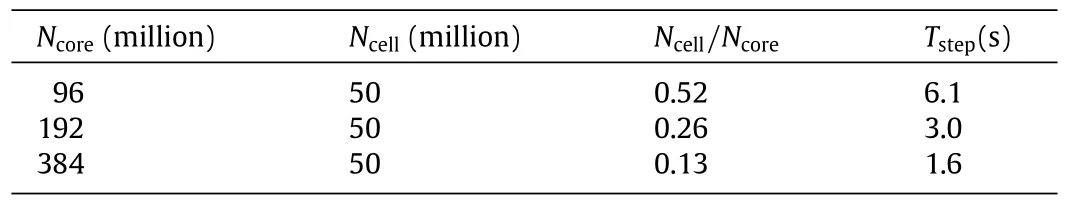
Table 1 Strong scalability of the flow solver on a mesh of about 50 million cells.The notations‘Ncore’and‘Ncell’denote the number of cores and the number of cells, respectively.‘Tstep’denotes the wall-clock time cost per step.

Table 2 Weak scalability of the flow solver with a mesh of about 0.26 million cells per core. The notations‘Ncore’and‘Ncell’denote the number of cores and the number of cells,respectively.‘Tstep’denotes the wall-clock time cost per step.

The present work focuses on deep-submergence underwater vehicle,where the effects of free surface on the flows near the model are ignored.The flows around the model are governed by theNavier–Stokesequationsforsinglephaseincompressibleflows. The governing equations for large eddy simulation are given by where˜ui(i=1,2,3)and˜pare the filtered velocity components and pressure,respectively.The sub-grid stresses˜τijis represented by the wall-adapting local eddy-viscosity model withCw= 0.6[13].fi(i=1,2,3)are the volume forces that represent the effects of boundaries on the flows in the IB method.Re is the Reynolds number.

Equations(1)and(2)are discretized on a Cartesian Eulerian mesh and solved by using a projection method.The secondorder central difference is used for the spatial derivatives,and the second-order Adams–Bashforth method is used for the time advance.Figure 1 presents the Lagrangian mesh near the sail and fins on the SUBOFF.A diffuse interface IB method based on the moving-least-squares reconstruction is used to represent the effects of the model surface on flows.[14,15].The computational domain is[-4.3D,4.3D]×[-4.3D,4.3D]×[-2.6D,23.2D].The uniformupstreamflowboundaryconditionisusedattheinlet,and convective outflow boundary condition is used at the outlet.The non-slip boundary conditions are used on the immersed surfaces. The slip boundary conditions are used at the outer boundaries.A trip wire is located at the 0.25Ddownstream of the model nose. The Reynolds number based on the upstream flow velocity and the length of the model isReL=U∞L/ν=1.0×105,corresponding to a Reynolds number based on the maximum diameter ofReD=U∞D/ν≈ 1.16×104.HereU∞is the uniform free stream flow velocity andνis the kinematic viscosity of the fluid.

In the present simulation,we utilize the block-structured mesh with adaptive mesh refinement.The parallel scalability of the flow solver is tested on meshes with different levels of refinement. Table 1 gives the wall-clock time cost of the flow solver on a mesh of about 50 million cells,which decreases as increasing the number of cores;Table 2 gives the wall-clock time cost of the flow solver on a mesh of about 0.26 million cells per core,which keeps nearly constant as increasing the number of cores.They show the strong and weak scalabilities of the parallel solver,respectively. In this letter,we report the preliminary results on the mesh of 50 million cells with a minimum grid length ofdh=0.0336. The minimum grid length is about 300 wall units,where the wall unit is estimated based on the turbulent boundary layer over a flat plate.The grid independence is checked to guarantee the sufficient resolution for the time-averaged pressure coefficient on the hull and the streamwise velocity profiles in the wake.It is worth to mention that the grid resolution is not fine enough to directly calculate the wall shear stress.A wall model is usually utilized to correctly obtain the wall shear stress in the LES with such a near-wallgridresolution.Wecalculatethetime-averagedpressure coefficient on the hull and the streamwise velocity profiles in the wake in the present letter.The simulations with wall models and the distribution of wall shear stress will be carried on in future.

Fig.2.(Color Online)The snapshots of the instantaneous vorticity magnitude(a,c)and pressure(b)at the symmetric plane(x=0).The notations‘TV’and‘BL’denote‘Tip Vortex’and‘Boundary Layer’,respectively.

Figure 2 plots the contours of vorticity magnitude and pressure at the symmetric plane(x=0).The essential features of flows can be observed,such as boundary layer,tip flows,shear layers and their interactions:(1)the pressure increases in front of the hull due to the decreasing velocities near the stagnation point at the nose;(2)the boundary layer develops from the stagnation point. The flow separates at the trip wire and reattaches to the hull in the rear of the trip wire;(3)the boundary layer and upstream flows interact with the leading edge of the sail,which causes a local pressure peak in front of the sail;(4)the tip flow origins from the top of the sail and moves downstream in the form of tip vortex;(5)the tip vortex(denoted as TV in Fig.2)interacts with the boundary layer(denoted as BL in Fig.2)in the middle of the hull;(6)the adverse pressure gradient occurs near the stern due to the contraction of hull and contributes to the boundary layer separation;(7)the boundary layer from the hull interacts with the fins,resulting in local pressure peaks in front of the fins;(8)the free shear layers shed from the fins and the hull are convected downstream into the wake;(9)the bimodal behavior of vorticity magnitudes can be observed in the wake,which is caused by the boundary layer separation and the interactions of the shear layers from both hull and fins.The pressure is consistent with the observed vortex structures[11,16,17],which can be found in the discussion on Fig.3.

The distributions of the time-averaged pressure coefficients at the bottom and top meridians of the model are shown in Fig.3.The pressure coefficient is computed in terms of

Fig.3.(Color Online)Time-averaged pressure coefficients on the top and bottom meridians of the model.

where˜p∞and 0.5ρU2∞are the static and dynamic pressures at the inlet,respectively.ρis the density of the fluid.The overall distribution of the time-averaged pressure coefficient is consistent with the experimental result of Jiménez et al.[16]and the numerical simulation of Posa and Balaras[11].The differences between the current simulation and the Refs.[11,16]are caused by the different Reynolds numbers.The Reynolds number in the present simulations isReL=U∞L/ν= 1.0× 105,which is only about 1/10 of those from the experiment(ReL=U∞L/ν= 1.1×106)[16]and the numerical simulation(ReL=U∞L/ν= 1.2×106)[11].The detailed features of the pressure coefficient are as follows:(1)the pressure coefficient has a maximum value at the stagnation point(z/L=0),and decreases sharply before it reaches the trip wire(0 ＜z/L＜ 0.03);(2)the pressure coefficient increases in the rear of the trip wire,and reaches a local maximum at the top meridian in front of the sail(0.03＜z/L＜ 0.2).The present simulation has a lower pressure region right behind the trip wire.The low pressure is caused by the size of the trip wire,in addition to the low Reynolds number effects.The diameter of the trip wire in the present simulation is about 10 times as large as those in the previous experiment and numerical simulation[11,16],which ensures the boundary layer transition at a lower Reynolds number;(3)the pressure coefficient at the bottom meridian varies slowly in the middle of the hull(0.2 ＜z/L＜ 0.7),since there is a parallel section in the model;the pressure coefficient at the top meridian varies slowly only in the region 0.4＜z/L＜ 0.7,because the wake of sail affects the pressure beforez/L=0.4;(4)The adversed pressure gradient appears near the stern(0.7 ＜z/L＜ 0.9). The pressure coefficient near the stern is higher than those in the Refs.[11,16].This is caused by the lower Reynolds number in the present simulation.The lower Reynolds number is corresponding to a thicker boundary layer along the hull.The thicker boundary layer reduces the effect of the geometry contraction of the hull; (5)the pressure coefficient reaches the local peak in front of the fins(z/L≈0.9),which corresponds to the interaction of boundary layers with fins.Notice that no fin is used in the experiment[16]. Instead, the full appendages are used in the present simulation.We also checked the effect of refinement levels on the distribution of pressure coefficients.The results show that the diffuse interface IB method reproduces the essential features of the distribution of pressure coefficient.

Figure 4 plots the time-averaged streamwise velocity profiles in the wake.The time-averaged streamwise velocity is normalized bythelocaldefectvelocityu0andhalf-wakewidthl0,whichsatisfy the following power law[18],respectively,

Fig.4.(Color Online)Self-similar behaviors of the time-averaged streamwise velocity profiles in the wake.The labels‘6D’,‘9D’,and‘12D’indicate the velocity profiles at 6D,9D,and 12D downstream from the model tail.

whereA,B,andx0are the coefficients dependent on the behaviors of the flow.The coefficients in Eqs.(4)and(5)for the present simulations areA=0.902,B=0.245,andx0=1.908.The velocity defects at three different locations in the wake are selfsimilar,since they nearly collapse into one single curve at the scaled vertical distances.The time-averaged velocity profile in the side of the sail(y/l0＞0)is lower than that in the experiment[16]. The lower time-averaged velocity profile is also reported by Posa and Balaras[11].This is caused by the blockage of the support in the experiment, since a long sail to support the model is used in the experiment.The time-averaged velocity defects without the effect of support are obtained by Jiménez et al.[16]and an analytical model for the axisymmetric wake provided by Pope[19]are also plotted in Fig.4.The velocity defects in the present simulation are consistent with the experimental and analytical results.

In summary,the large eddy simulation of DARPA SUBOFF with the full appendages is performed by using a diffuse interface immersed boundary method.Particularly,the IB method is implemented through the moving-least-squares reconstruction and the block structured meshes with adaptive mesh refinement. The parallel scalabilities of the flow solver are tested on meshes at different levels of refinement with the total cells number varying from 50 million to 3.2 billion.It is shown that the parallel solver has the nearly linear strong and weak scalabilities for the present configuration.The numerical results provide the overall features of the flows near the hull surfaces and in the wake. The time-averaged pressure coefficients on the hull surface are consistent with the model configuration.The defects of time-averaged streamwise velocities exhibit the self-similarities as predicted by the power law.

The diffuse interface IB method used in this work is robust and efficient for simulating intermediate Reynolds number flows aroundunderwatervehicles.However,itremainsagreatchallenge that the IB method is used to predict the shear stresses on hull surfaces.The shear stresses are dependent on the velocity gradients near surfaces so that the finer meshes in the wallnormal direction are needed.It is noted that the meshes in the IB method cannot be refined only in the wall-normal direction. Two possible approaches to overcome this defeat are to increase the grid numbers near wall and use the wall models.The nearly linear scalability of the present flow solver allows us to use tens of thousands of cores with billions of grid points in National Center of Supercomputer.Meanwhile,we will use the wall models for the IB method to reduce the computational cost and provide a feasible approach for the simulation-based studies of underwater vehicles.

Acknowledgments

This work was supported by the National Natural Science Foundation of China(11302238,11232011 and 11572331).The authors would like to acknowledge the support from the Strategic Priority Research Program(XDB22040104)and the Key Research Program of Frontier Sciences of the Chinese Academy of Sciences (QYZDJ-SSW-SYS002)and the National Basic Research Program of China(973 Program 2013CB834100:Nonlinear science).

[1]P.R. Bandyopadhyay, Trends in biorobotic autonomous undersea vehicles, IEEE J. Ocean. Eng. 30 (2005) 109–139

[2]X.C. Wu, Y.W. Wang, C.G. Huang, et al., An effective CFD approach for marine-vehicle maneuvering simulation based on the hybrid reference frames method, Ocean Eng. 109 (2015) 83–92.

[3]Y.Yang,D.I.Pullin,Evolution of vortex-surface fields in viscous Taylor-Green and Kida-Pelz flows,J.Fluid Mech.685(2011)146–164.

[4]Y.M.Zhao,Y.Yang,S.Y.Chen,Vortex reconnection in the late transition in channel flow,J.Fluid Mech.802(2016)R4.http://dx.doi.org/10.1017/jfm. 2016.492.

[5]J.M.Yang,E.Balaras,An embedded-boundary formulation for large-eddy simulation of turbulent flows interacting with moving boundaries,J.Comput. Phys.215(2006)12–40.

[6]X.L.Yang,G.W.He,X.Zhang,Large-eddy simulation of flows past a flapping airfoil using immersed boundary method,Sci.China Phys.Mech.Astron.53 (2010)1101–1108.

[7]C.Yan,W.X.Huang,G.X.Cui,et al.,A ghost-cell immersed boundary method for large eddy simulation of flows in complex geometries,Int.J.Comput.Fluid Dyn.29(2015)1–14.

[8]C.S.Peskin,The immersed boundary method,Acta Numer.11(2001)479–517.

[9]R.Mittal,G.Iaccarino,Immersed boundary methods,Annu.Rev.Fluid Mech. 37(2005)239–261.

[10]F.Sotiropoulos,X.L.Yang,Immersed boundary methods for simulating fluid–structure interaction,Prog.Aerosp.Sci.65(2014)1–21.

[11]A.Posa,E.Balaras,A numerical investigation of the wake of an axisymmetric body with appendages,J.Fluid Mech.792(2016)470–498.

[12]N.C.Groves,T.T.Huang,M.S.Chang,Geometric Characteristics of the DARPA SUBOFF Models,Tech.Rep.No.DTRC/SHD-1298-01,David Taylor Research Center,Bethesda,MD,1989.

[13]F.Nicoud,F.Ducros,Subgrid-scale stress modelling based on the square of the velocity gradient tensor,Flow Turbul.Combust.62(1999)183–200.

[14]M.Vanella,P.Rabenold,E.Balaras,A direct-forcing embedded-boundary method with adaptive mesh refinement for fluid–structure interaction problems,J.Comput.Phys.229(2010)6427–6449.

[15]M.Vanella,E.Balaras,A moving-least-squares reconstruction for embeddedboundary formulations,J.Comput.Phys.228(2009)6617–6628.

[16]J.M.Jiménez,R.T.Reynolds,A.J.Smits,The intermediate wake of a body of revolution at high Reynolds numbers,J.Fluid Mech.659(2010)516–539.

[17]J.M.Jiménez,R.T.Reynolds,A.J.Smits,The effects of fins on the intermediate wake of a submarine model,J.Fluids Eng.132(2010)031102.

[18]P.B.V.Johansson,W.George,M.Gourlay,Equilibrium similarity,effects of initial conditions and local Reynolds number on the axisymmetric wake,Phys. Fluids 15(2003)603–617.

[19]S.B.Pope,Turbulent Flows,Cambridge University,United Kingdom,London, 2010(Chapter 5).

∗Corresponding author.

E-mail address:hgw@lnm.imech.ac.cn(G.He).

http://dx.doi.org/10.1016/j.taml.2016.11.004

2095-0349/©2016 The Authors.Published by Elsevier Ltd on behalf of The Chinese Society of Theoretical and Applied Mechanics.This is an open access article under the CC BY-NC-ND license(http://creativecommons.org/licenses/by-nc-nd/4.0/).

*This article belongs to the Fluid Mechanics