Study of fluid resonance between two side-by-side floating barges*

Xin LI （李欣）， Liang-yu XU （徐亮瑜）， Jian-min YANG （杨建民）

1. State Key Laboratory of Ocean Engineering， Shanghai Jiao Tong University， Shanghai 200240， China

2. Collaborative Innovation Center for Advanced ship and Deep Sea Exploration Shanghai 200240， China，E-mail: lixin@sjtu.edu.cn

3. Department of Mechanical Engineering， Massachusetts Institute of Technology， Cambridge， MA， USA

Study of fluid resonance between two side-by-side floating barges*

Xin LI （李欣）1，2， Liang-yu XU （徐亮瑜）3， Jian-min YANG （杨建民）1，2

1. State Key Laboratory of Ocean Engineering， Shanghai Jiao Tong University， Shanghai 200240， China

2. Collaborative Innovation Center for Advanced ship and Deep Sea Exploration Shanghai 200240， China，E-mail: lixin@sjtu.edu.cn

3. Department of Mechanical Engineering， Massachusetts Institute of Technology， Cambridge， MA， USA

The hydrodynamic interaction between two vessels in a side-by-side configuration attracted research attentions in recent years. However， because the conventional potential flow theory does not consider the fluid viscosity， in the hydrodynamic results， the wave elevations were overestimated in the narrow gap under resonance conditions. To overcome this limitation and investigate the complex fluid flow around multiple bodies in detail， this study examines the fluid resonance between two identical floating barges using a viscous flow analysis program FLOW-3D. The volume of fluid method is implemented for tracking the free surface， and a porous media model is used near the outflow boundary to enhance the wave absorption. A three-dimensional numerical wave basin is established and validated by comparison with the waves generated using theoretical values. On this basis， a computational fluid dynamics （CFD） simulation of the two barges in a resonance wave period is performed， and the wave elevations， the fluid flow around the barges， and the motions of the barges are discussed. The numerical simulation is verified by comparison with results of corresponding experimental data.

side-by-side bodies， FLOW-3D， wave elevation， streamline， fluid resonance

Introduction

The rapid progress in the exploitation of ocean resources along with the escalation in oil prices and the demand for natural gas involves the use of numerous facilities and operations of multiple floating bodies. Examples include the floating liquefied natural gas （FLNG） offloading， the topside floatover installation for a platform［1］， and a multiple-body mobile offshore base （MOB）［2］. Hydrodynamic interactions between multiple bodies greatly affect their motion responses and wave forces， and it is particularly significant to understand these interactions for ensuring safe operations in practical engineering.

The hydrodynamic interactions between floating bodies were extensively studied， including numerical simulations based on the linear 3-D potential flow theory［3-5］or model test studies［6，7］for two-body hydrodynamic interactions. However， with the potential flow theory， the fluid viscosity is ignored， and therefore，when the bodies are in close proximity， unrealistically high free surfaces appear in the gap between the bodies under resonance conditions in the numerical simulations. in the hydrodynamic results， the wave elevations were overestimated by the potential flow theory. Therefore， recent research attempts were focused on improving the available numerical methods for making realistic predictions of the free-surface elevation. Huijsmans et al.［8］incorporated a rigid lid on the free surface between two vessels to suppress the unrealistic resonant wave oscillation. Further， Newman［9］presented a suppression method based on the damping of generalized motion modes. Fournier et al.［10］made a pioneering attempt to apply a new damping lid method［11］to multi-body hydrodynamics， in which a damping lid was applied to the free surface between two bodies to reduce the wave elevation and drift forces.

In these improved methods， corresponding model tests must be carried out to provide data for calibration and the selection of damping values， however， these tests are expensive and time consuming， and they require large model basins， further， they may not always be possible to perform. The use of the computationalfluid dynamics （CFD） is a new approach for investigating the fluid resonance in the narrow gap between multiple bodies. For example， Sauder et al.［12］used a Navier-Stokes solver to investigate the gap-resonance problem between a bottom-mounted offshore terminal and a nearby LNG carrier in a 2-D setting. Lu et al.［13，14］employed 2-D viscous fluid models to study the fluid resonance in the two gaps between three fixed bodies and the wave forces on them， with considerations of different gap widths， body drafts， body breadth ratios， and body numbers for performing sensitivity analyses of wave forces.

However， these studies of voscosity as described above were limited to 2-D models， to the best of the authors' knowledge， no studies have considered 3-D models， probably because of the complexity of the multi-body problem and the high computational cost for 3-D models. However， the use of 3-D models is desirable because a 3-D simulation enables a detailed observation as well as the revelation of the basic physics of multi-body interaction. Therefore， this study investigates the fluid resonance between two adjacent identical floating barges using a viscous flow analysis program FLOW-3D， an effective viscous simulation tool. This software was previously employed by Muk-Pavic et al.［15］and Lee et al.［16］in their studies of LNG tank sloshing loads and free-surface flow around the ship hull， respectively.

1. Mathematical formulations

1.1Fluid flow governing equations

Assuming an incompressible and Newtonian fluid，in a laminar flow， and with a constant viscosity， the governing equations for the fluid flow are the mass continuity equation and the momentum equations:

where U=（u，v，w）is the fluid velocity， ρ is the fluid density， p is the fluid pressure， g is the gravity and noninertia body acceleration， and =/νμρ is the kinematic viscosity. F denotes other forces， such as the wall shear stresses at solid boundaries and the resistance force in a porous medium.

1.2Free-surface model and porous media model

The volume of fluid （VOF） method［17］is used for tracking the free surface， where a VOF function （，Fx，，）yzt is introduced to define the fluid configurations. In a “one-fluid” model， the air is treated as a void and the free surface is an external boundary with uniform pressure across the interface. In this case， F represents the volume fraction occupied by the fluid and satisfies the following transport equation

A porous media model is defined for the wave absorption near the outflow boundary. The resistance to the flow in a porous medium is represented in the momentum equations as a drag term proportional to the velocity

wheredF is the drag coefficient in the porous media. The Forchheimer model is used for simulating the porous media containing coarse particles， in this case， Fdis expressed as

where a=180/D2and D is the particle diameter， Vfis the volume fraction in the fractional area/volume obstacle representation （FAVOR） method， which is used for defining the solid boundary within the Eulerian grid and is based on the concept of the area fraction （Af） and the volume fraction （Vf） open to the flow on a rectangular structured mesh. In a porous medium，fV is identical to the porosity［18］.

1.3Moving object model

The general moving object （GMO） model is used to simulate the motions of the two barges. The motions in the horizontal directions （sway， surge， and yaw） are constrained to fix the barges' positions， and the vertical motions in the other three degrees of freedom （DOF），i.e.， heave， pitch， and roll， are dynamically coupled with the fluid flow. For the coupled motions， at each time step， the hydraulic， gravitational， and inertial forces and torques are calculated and the motion equations are solved. A body-fixed coordinate system with respect to the center of gravity （COG） is set for each GMO. Based on Newton's second law， the 3-DOF motion equations in the vertical direction for each rigid body can be expressed as

whereZF，GxT andyGT are the external force and moments in corresponding directions， m is the body mass，xxI andyyI are the moments of inertia， andGZV is the velocity of the COG in the z direction.

To account for the effect of the moving objects to displace the fluid， source terms are added to the continuity equation （Eq.（1）） and the VOF transport equation （Eq.（3））. At each time step， the area and volume fractions are recalculated on the basis of the updated barge locations and orientations； the fluid and GMO motions are calculated iteratively by an implicit method.

1.4Boundary conditions

The initial conditions are the still water with a zero velocity and a hydrostatic pressure distribution. In general， the boundary conditions represent the external factors in a flow problem. In the case of waves propagating in a wave basin， the boundary conditions are as follows:

（1） On the inflow boundary， a periodic linear surface wave is generated based on the Airy's linear wave theory. More details can be found in the reference［19］.

（2） On the outflow boundary， the Sommerfeld radiation boundary condition is adopted and a mathematical continuation of the flow beyond the end of the wave basin is assumed， which takes the form of the outgoing waves

where Q is any quantity， c is the local phase speed of the assumed wavelike flow， and the positive x is pointed out of the boundary.

（3） On the symmetry boundary， all scalars have zero gradients. The normal velocity and flux through the boundary are both zero. The normal gradient of the tangential velocity components is also zero， which means that the shear stresses disappear.

（4） On the wall boundary， the velocity and the convective fluxes are zero， a no-slip boundary condition is imposed for accounting for the wall shear stresses， the pressure is set as having a zero normal gradient.

（5） On the free-surface boundary， the pressure（normal stress） is specified. All velocity derivatives that involve the velocity components outside the surface are set to zero to ensure zero tangential stress.

（6） On the solid body boundary， a no-slip boundary is prescribed， where the normal velocity is equal to the body velocity and the tangential velocity is set to zero. The pressure is set as having a zero normal gradient.

1.5Numerical method

In the FLOW-3D， a finite difference approach is used for discretization of the computational domain. For the spatial discretization of the momentum equations （Eq.（2））， the first-order upwind and second-order central-difference approximations are combined into a single expression， with an adjusting parameter to discretize the advection term. The viscous shear term is discretized using a standard second-order centraldifference scheme. A semi-implicit scheme is applied for the time advancement， in which most terms are evaluated explicitly but the pressure and the velocity are coupled implicitly. The discretized forms of the governing equations for the fluid flow are as follows，with considerations of the FAVOR method， the porous medium model， and the wall shear stresses at the wall boundary and the solid body boundary.

where AFRi-1，j，kis the area fraction between meshes（i，j，k） and （i+1，j，k）， AFBi，j，kis the area fraction between meshes （i，j，k） and （i，j+1，k）， and AFTi，j，kis the area fraction between meshes （，，）ijk and （，i j，k+1）. FU（U，W）， X（X，Y）， VISX（Y，Z） and WSX（Y，Z） denote the convection fluxes， the acceleration due to the internal viscous shear， and the acceleration due to the wall shear stress， respectively［20］.

The pressure gradient is isolated from the other terms in the momentum equations by using the fractional-step method. The resulting pressure-Poisson equation is solved using the generalized minimal residual （GMRES） algorithm.

Fig.1 Sketch of the numerical wave basin

Fig.2 Mesh distributions of the numerical basin

2. Numerical simulation

2.1Numerical wave basin and its validation

The dimensions of the numerical wave basin are 7.5 m×3 m×0.9 m and the water depth is set as 0.7 m，with considerations of the main parameters of the two barges in the model scale. The origin is set at the stillwater surface at the left end of the basin， as shown in Fig.1. We use a mesh of 800 cells uniformly distributed in the x direction， varied grade of 200 and 102 cells in the y and z directions， respectively. A dense mesh system is adopted near the still-water surface and the gap between the two barges， the mesh distributions in the -xz and -yz planes are illustrated in Fig.2. The time step is adjusted by changing the Courant number.

The inflow and outflow boundary conditions are set on the left and right ends， respectively， of the numerical basin. The incident wave is a regular wave with wave amplitude A of 0.0175 m and period T of 0.6455 s， which is a third-order Stokes wave. The wall boundary condition is imposed at the bottom， and the symmetry boundary condition is imposed on the two sidewalls of the numerical wave basin. At the free surface， the pressure is set as 1.01×105Pa. A sloping porous media model is applied near the outflow boundary to supplement the wave absorption and minimize the wave reflection. The slope factor is 1:3， and the porosity is 0.8.

Fig.3 Time series of wave elevation at =2mx， =0y （model scale）

Fig.4 Wave elevation and pressure distribution at =12st（model scale）

A regular wave test is performed for validating the wave generation in the 3-D numerical wave basin. After about 10 s of calculation， a stable pattern of the wave emerges. The resulting time series of the wave elevation at x=2m， y=0 and t=12s-16s （in model scale） is presented in Fig.3， where η is free-surface elevation， t is time， the figure also shows its comparison with corresponding values obtained from the third-order Stokes wave theory. It can be seen that the calculated results are in good agreement with the theoretical ones. Figure 4 shows the wave elevation and the pressure distribution in the entire computational domain at =12st， the wave distribution is stable and almost perfect， which satisfies the requirement for the accurate generation of waves.

2.2CFD Simulation of two side-by-side barges with a narrow gap

Barge BH222 and barge BH223， developed by the China Offshore Oil Engineering Corporation（COOEC）， are arranged side by side， they are selected as a reference. They were designed to be used in a floatover installation of a jacket platform in China's Bohai Sea at a water depth of 42 m. The two barges are identical， with the same weight and dimensions. The main parameters of the two barges and the corresponding model values with a scale of 1:60 are listed in Table 1. The gap width between the two barges is set to be 3 m in the full scale， which is the closest to the gap in the floatover operation.

Table 1 Main parameters of barge BH222 and barge BH223

First， the hydrodynamic performances of the two barges with a 3 m gap and the wave elevation around the barges are studied using the potential flow theory in the full scale. The calculated results in the frequency domain under a head sea condition are compared with the corresponding experimental values determined from white noise wave tests （Fig.5）. Tw is wave period. The comparison shows that the calculated results agree well with the experimental results， except for a difference in the peak values near the resonance period （5 s）. This difference may be attributed to the fact that the fluid viscosity is not considered in the potential flow theory. Therefore， a viscous flow model is adopted to account for the viscous dissipation and also to investigate in detail the underlying principle and mechanism of the multi-body interaction.

Fig.5 Wave elevation at the center of the gap （Point C， full scale）

Next， a CFD simulation of the fluid flow around the two side-by-side barges is performed. The horizontal motions （surge， sway and yaw） of the two barges are fixed to maintain its position constant， and the vertical motions are dynamically coupled with the fluid flow. A model system is adopted for comparison with the model test. The two barge models with a 1:60 model scale are added to the above numerical wave basin， with their bows being located 3 m from the left boundary （Fig.6）. The wave period of 0.6455 s corresponds to the actual wave period of 5 s， which is the resonance period； the wave height is defined as 0.035 m. The simulation starts from a stable wave state， =12st in the above-described wave validation study with no barges.

Fig.6 Numerical wave basin with two side-by-side barges

3. Experimental study

To verify the numerical results of the fluid flow and the wave elevation in the gap， corresponding model tests are carried out in the basin at the StateKey Laboratory of Ocean Engineering （SKLOE） at Shanghai Jiao Tong University， China. The model scale is 1:60. The dimensions of the basin are 50 m× 30 m×6 m， and the water depth is set to 0.7 m， which corresponds to the actual water depth of 42 m.

In the model tests， the horizontal motions of the two barge models are controlled using a mooring system modeled by four wire springs on each barge， as shown in Fig.7. The angles between the spring lines and the x axis are adjusted too45， and the pre-tensions acting on each mooring line are about 5 N in the model scale.

Fig.7 Mooring configuration of two side-by-side barges （model scale）

Fig.8 Test setup for the two barges

Then， regular head wave tests for the two sideby-side barge models with a 0.05 m gap （3 m in full scale） are carried out. The wave height and period are 0.035 m and 0.6455 s （2.1 m and 5 s in the full scale），respectively. It is observed that the fluid flow is violent in the gap between the two barges， and the gap size obviously is increased. The gap size has a strong influence on the fluid flow and the barge motions， therefore， two hinged wire lines are added at the bow and the stern to connect the two barges and to maintain the 0.05 m distance constant. White noise wave tests under the head sea condition are also performed. The periods cover a large interval of 5 s-20 s with a wave height of 3 m in the full scale. The response amplitude operator（RAO） is obtained through spectral analysis.

The wave elevations in the gap are measured using resistance probes at five locations: midship and ±0.25m and ±0.50m from the midship （Points A-E in Fig.7） in the model scale. The motion responses of the two barges are recorded by noncontact laser position finders. The test setup is shown in Fig.8. A camera is used to observe the fluid flow around the two barges.

Fig.9 Wave elevation at Point A （model scale）

Fig.10 Wave elevation at Point B （model scale）

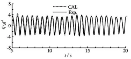
Fig.11 Wave elevation at Point C （model scale）

4. Results and discussions

4.1Wave elevations around the two barges

The calculation results by using the potential flow theory show that the fluid flow in the gap is extremely violent. Therefore， the time series of the wave elevations are recorded at five locations in the gap andcompared with the corresponding results of the regular head wave test， as shown in Figs.9-13. In these figures，the ordinate represents the dimensionless wave elevation， which is obtained by dividing the free-surface elevation η by the incident wave amplitude A. In the calculated results， a stable pattern is reached after about 8 s. The wave elevations at Points B and C are larger than those at other locations， and the maximum wave elevation could reach up to over four times the incident wave amplitude， which indicates the violent fluid flow in the gap. Comparison with the model test values shows that the results of the viscous flow simulation and the experiment are generally in good agreement， except for the calculated wave elevation at Point D， which is larger than the corresponding experimental value. This difference may be attributable to the different levels of constraints for horizontal motions: in the numerical simulation， the horizontal motions of the two barges are completely constrained， whereas in the experiment， they are partly confined by eight wire springs. From the research of Sun et al.［21］， it is known that the locations of the peaks are strongly dependent on whether the bodies are fixed or freely floating.

Fig.12 Wave elevation at Point D （model scale）

Fig.13 Wave elevation at Point E （model scale）

Fig.14 Wave elevations around the two barges in a period（model scale）

Figure 14 shows the wave elevations around the two barges in a typical regular wave period （=t 13.36s-14.00s）. The wave field is seen visibly to curl near the front and trailing ends of the gap. At the beginning of a period， the maximum wave elevation appears before the bows of the two barges， and its value of 0.0374 m is essentially equal to twice the incident wave amplitude， this large elevation results from the superposition of the incident wave and the wave reflected from the bows. At time =1/4tT， large wave amplifications occur at the center of the gap near Points B and C， and the maximum wave elevation of 0.068 m is the largest value in a period. Right in the middle of a period （t=1/2T）， the wave elevations inthe gap decrease and the maximum value is reached at the front end of the gap. This simulation result is consistent with the model test observation， in the regular wave test， it is found that the fluid flow is complex and violent at the front end of the gap， in addition to being that way in the midgap. However， this behavior is not observed in the potential flow calculation results，so no such wave probe is set in the experiment. No such or similar behavior is observed in previous studies， so we ascribe it to the shapes of the bows of the barges. At time =3/4tT， the wave elevation in the midgap reaches its minimum value， and no obvious wave amplification region is visible around the two barges. At the end of a period， the wave elevation returns to its state at the start of the period， and the above process is repeated all over again.

Figure 15 shows the wave elevations along the x axis of the numerical wave basin at plane =0y and times =1/4tT and =3/4tT. The two red dashed lines represent the positions of the barge bow and stern，and it can be clearly seen that because of the hydrodynamic interaction between the two barges， the wave in the gap exhibits a resonance behavior with a large wave elevation and a strong fluid oscillation （Fig.16）. After the wave propagates to the trailing end of the gap，the free-surface elevation decreases rapidly and remains stable until it is absorbed at the right end of the numerical wave basin.

Fig.15 Wave elevations along the x axis of the numerical wave basin （model scale）

Fig.16 Wave elevations around the two barges at =1/4tT

Fig.17 Instantaneous streamlines on the free surface around the barges

4.2Fluid flow in the gap

For further insights into the structure of the fluid flow， a sequence of instantaneous 3-D streamlines on the free surface around the two barges are shown in Fig.17 and Fig.18， respectively， as well as the pressure and velocity distributions on the transverse section of the midship （x=3.75m） in a regular wave period. The states of the fluid flow at the start and the end of a period are identical， so the results at time t=T are not shown here. At the beginning of a period， the fluid flows into the gap from under the barge bottoms， and atthe fro nt par t unde r eachbarg e， the re app earsto be asourcepointfromwhichthefluidflowsout.Theupward velocity of the fluid in the gap contributes to the increasing wave elevation， which attains its maximum at time =1/4tT. At this moment， the velocity starts to change its direction and the downward velocity emerges and increases gradually. The streamline pattern at time =1/4tT shows that after the maximum elevation is reached， the fluid in the midgap starts flowing forward or backward in the gap or toward the barge bottoms， and at the trailing end of the gap， some fluid starts flowing into the gap from behind the barges. At time =1/2tT， the downward velocity in the gap attains its maximum value and the free surface is essentially at its static equilibrium position， at the front part under each barge， there appears to be a sink point collecting fluid from different locations. At time =t 3/4T in the midgap， the free elevation is the lowest and the downward fluid velocity reduces to zero and reverses its direction to become upward. The fluid flow close to the barge hull has an upward velocity component （Fig.18（d）） and the fluid under the barges flows toward the gap， which leads to an increase of the wave elevation in the gap， causing the overall behavior of the fluid to become similar to that at the start of a period.

Fig.18 Pressure and velocity distributions in the transverse section of midship （model scale）

4.3Barge motions in waves

The time series of the heave， roll， and pitch motions for the two barges in the viscous simulation are shown in Figs.19-21， where3X is heave，4X is roll，and5X is pitch. It can be observed that the two barges have essentially the same heave and pitch motions owing to their symmetrical positions relative to the incident wave. Similar to the calculated time series of the wave elevation， the motion results also attain stability after about 8 s. The evident roll motion begins at about 4 s and then increases gradually， from 8 to 13 s，the roll motions of the two barges share the same period with a phase difference of π， which implies that their roll motions have opposite directions. This phenomenon is consistent with the experimental observation.

Fig.19 Time series of heave motion （model scale）

Fig.20 Time series of roll motion （model scale）

Fig.21 Time series of pitch motion （model scale）

Fig.22 Motion RAOs from white noise wave tests （full scale）

Motion RAOs for the barges from the white noise wave tests are shown in Fig.22， these results are in the full scale. When the incident wave period is 5 s（0.6455 s in the model scale）， the heave， roll， and pitch RAOs in the full scale are 0.0117， 0.218o/m， and 0.267o/m， respectively， the corresponding simulation values are 0.002 m， 0.229o， and 0.280o， respectively. Comparison with the above time series shows that the pitch motion sees a good agreement， while large discrepancies exist in the results of the heave and roll motions. In the simulation， the heave motion is overestimated and the roll motion is much larger. The reason for these discrepancies is probably the fixed horizontal motions of the barges in the viscous simulation. The motion RAOs of freely floating barges are compared with those of barges with no horizontal motions using the potential flow theory， as shown in Fig.23，and it is found that the fixation on horizontal motions has a significant influence on the motion responses. At a wave period of 5 s in the full scale， all vertical motions for the barges with no horizontal motions are greater than those for the freely floating barges， this is especially the case for the roll motion.

Fig.23 Motion RAOs from potential flow calculation （full scale）

5. Concluding remarks

This study investigates the fluid resonance in the narrow gap between two floating barges using a viscous flow analysis program FLOW-3D. The vertical motions of the two barges are dynamically coupled with the fluid flow. A 3-D numerical wave basin is built and the generated wave is validated through comparison with theoretical values. On this basis， two sideby-side barges are added to the numerical wave basinfor the CFD simulation， the wave and multi-body interaction is modeled and simulated. Corresponding model tests are carried out as a reference for verification of the numerical simulation.

Comparison between the computational and experimental results demonstrates that the CFD simulation performed in this study is capable of simulating the wave elevation around the two barges. Therefore， the CFD simulation may provide an alternative approach when corresponding experiments are not performed. The detailed investigation of the fluid flow around the two barges in a regular wave period shows that the excitation of the wave amplification in the gap is induced mainly by the fluid flow under the barge bottoms rather than by a standing wave resulting from the superposition of incident and diffracted waves. The hydrodynamic interaction of multiple bodies is a very complex process， the fluid flow is difficult to observe and analyze by an experimental method. However， the viscous simulation performed in this study enables a detailed observation and analysis of the fluid flow around multiple bodies， which helps the elucidation of the mechanism of the multi-body interaction. The 3-D CFD simulation provides new insights into the fluid and multi-body interaction.

Acknowledgement

This work was supported by the Youth Innovation Fund of the State Key Laboratory of Ocean Engineering， Jiao Tong University （Grant No. GKZD010059-21）.

References

［1］XU Xin， YANG Jian-min and LI Xin et al. Time-domain simulation for coupled motions of three barges moored side-by-side in floatover operation［J］. China Ocean Engineering， 2015， 29（2）: 155-168.

［2］SUZUKI H.， RIGGS H. R. and FUJIKUBO M. et al. Very large floating structures［C］. ASME 2007 26th International Conference on Offshore Mechanics and Arctic Engineering. San Diego， California， USA， 2007， 597-608.

［3］FANG M. C.， CHEN G. R. On three-dimensional solutions of drift forces and moments between two ships in waves［J］. Journal of Ship Research， 2002， 46（4）: 280-288.

［4］MING Ping-jian， ZHANG Wen-ping . Numerical method for multi-body fluid interaction based on Immersed Boundary Method［J］. Journal of Hydrodynamics， 2011， 23（4）: 476-482.

［5］XU Xin， LI Xin and YANG Jian-min et al. Hydrodynamic interactions of three barges in close proximity in a floatover installation［J］. China Ocean Engineering， 2016，30（3）: 343-358.

［6］HONG S. Y.， KIM J. H. and CHO S. K. et al. Numerical and experimental study on hydrodynamic interaction of side-by-side moored multiple vessels［J］. Ocean Engineering， 2005， 32（7）: 783-801.

［7］XU X.， YANG J. M. and LI X. et al. Hydrodynamic performance study of two side-by-side barges［J］. Ships and Offshore Structures， 2014， 9（5）: 475-488.

［8］HUIJSMANS R. H. M.， PINKSTER J. A. and De WILDE J. J. Diffraction and radiation of waves around side-byside moored vessels［C］. Proceedings of11th Internatinal Offshore and Polar Engineering Conference. Stavanger， Norway， 2001.

［9］NEWMAN J. N. Application of generalized modes for the simulation of free surface patches in multiple body hydrodynamics［C］. Proceedings of 4th Annual WAMIT Consortium Report. Woods Hole， MA， USA， 2003.

［10］ FOURNIER J. B.， NACIRI M. and CHEN X. B. Hydrodynamics of two side-by-side vessels， experiments and numerical simulations［C］. Proceedings of 16th International Offshore and Polar Engineering Conference. San Francisco， CA， USA， 2006.

［11］ CHEN X. B. Hydrodynamic analysis for offshore LNG terminals［C］. Procedings of 2nd International Workshop on Applied Offshore Hydrodynamics. Rio de Janeiro， Brazil. 2005.

［12］ SAUDER T.， KRISTIANSEN T. and OSTMAN A. Validation of a numerical method for the study of piston-like oscillations between a ship and a terminal［C］. Proceedings of 20th Internatinal Offshore and Polar Engineering Conference. Beijing， China， 2010.

［13］ LU L.， CHENG L. and TENG B. et al. Numerical investigation of fluid resonance in two narrow gaps of three identical rectangular structures［J］. Applied Ocean Research，2010， 32（2）: 177-190.

［14］ LU L.， TENG B. and SUN L. et al. Modelling of multibodies in close proximity under water waves-Fluid forces on floating bodies［J］. Ocean Engineering， 2011， 38（13）: 1403-1416.

［15］ MUK-PAVIC E.， CHIN S. and SPENCER D. Validation of the CFD code Flow-3D for the free surface flow around the ships' hulls［C］. 14th Annual Conference CFD Society of Canada. Kingston， Canada， 2006.

［16］ LEE D. H.， KIM M. H. and KWON S. H. et al. A parametric sensitivity study on LNG tank sloshing loads by numerical simulations［J］. Ocean Engineering， 2007， 34（1）: 3-9.

［17］ HIRT C. W.， NICHOLS B. D. Volume of fluid （VOF）method for the dynamics of free boundaries［J］. Journal of computational physics， 1981， 39（1）: 201-225.

［18］ FLOW-3D. User Manual （V.10.0）［R］. Flow Science Inc.，2011.

［19］ BASCO D. R. Water wave mechanics for engineers and scientists.eos［J］. Transactions American Geophysical Union， 1985， 66（24）: 490-491.

［20］ VANNESTE D. Experimental and numerical study of wave-induced porous flow in rubble-mound breakwaters［D］. Doctoral Thesis， Ghent， Belgium: Ghent University， 2012.

［21］ SUN L.， TAYLOR R. E. and TAYLOR P. H. First-and second-order analysis of resonant waves between adjacent barges［J］. Journal of Fluids and Structures， 2010， 26（6）: 954-978.

（October 11， 2014， Revised May 16， 2015）

* Project supported by the National Natural Science Foundation of China （Grant No. 51509152）.

* Biography： Xin LI （1975-）， Female， Ph. D.，

Associate Professor