Modelling of a non-buoyant vertical jet in waves and currents*

Zhen-shan XU （徐振山）， Yong-ping CHEN （陈永平）， Jian-feng TAO （陶建峰）， Yi PAN （潘毅），

Chang-kuan ZHANG （张长宽）2， Chi-Wei LI （李志伟）3

1. State Key Laboratory of Hydrology-Water Resources and Hydraulic Engineering， Hohai University， Nanjing 210098， China， E-mail: zsxu2006@ hhu.edu.cn

2. College of Harbor， Coastal and Offshore Engineering， Hohai University， Nanjing 210098， China

3. Department of Civil and Environmental Engineering， The Hong Kong Polytechnic University， Hong Kong，China

Modelling of a non-buoyant vertical jet in waves and currents*

Zhen-shan XU （徐振山）1，2， Yong-ping CHEN （陈永平）1，2， Jian-feng TAO （陶建峰）1，2， Yi PAN （潘毅）2，

Chang-kuan ZHANG （张长宽）2， Chi-Wei LI （李志伟）3

1. State Key Laboratory of Hydrology-Water Resources and Hydraulic Engineering， Hohai University， Nanjing 210098， China， E-mail: zsxu2006@ hhu.edu.cn

2. College of Harbor， Coastal and Offshore Engineering， Hohai University， Nanjing 210098， China

3. Department of Civil and Environmental Engineering， The Hong Kong Polytechnic University， Hong Kong，China

A generic numerical model using the large eddy simulation （LES） technique is developed to simulate a non-buoyant vertical jet in wave and/or current environments. The experimental data obtained in five different cases， i.e.， one case of the jet in a wave only environment， two cases of the jet in a cross-flow only environment and two cases of the jet in a wave and cross-flow coexisting environment， are used to validate the model. The grid sensitivity tests are conducted based on four different grid systems and the results illustrate that the non-uniform grid system C （205×99×126 nodes with the minimum size of 1/10 jet diameter） is sufficiently fine for the modelling. The comparative study shows that the wave-current non-linear interaction should be taken into account at the inflow boundary while modelling the jet in wave and cross-flow coexisting environments. All numerical results agree well with the experimental data， showing that: （1） the jet under the influence of the wave action has a faster centerline velocity decay and a higher turbulence level than that in the stagnant ambience， meanwhile the “twin peaks” phenomenon exists on the cross-sectional velocity profiles， （2） the jet under a cross-flow scenario is deflected along the cross-flow with the node in the downstream， （3） the jet in wave and cross-flow coexisting environments has a flow structure of “effluent clouds”， which enhances the mixing of the jet with surrounding waters.

large eddy simulation （LES）， turbulent jet， wave， cross-flow， wave and cross-flow coexisting

Introduction

The disposal of wastewater into coastal waters is one of common sewage treatment approaches in coastal cities. It is of importance to understand and predict the movement of the disposed wastewater， which is usually in the form of a turbulent jet， in order to make a more accurate assessment of the wastewater impact on the surrounding environment. In coastal waters， the jet is not only driven by its initial momentum， but also affected by the coastal hydrodynamics， such as tidal currents and/or waves. If the jet is vertically discharged into the ambience， the surrounding tidal currents could be approximated as a series of quasi-steady cross-flows.

Many experiments were carried out to investigate the vertical jet in either the cross-flow or the wave environment. A better understanding of the complex interaction mechanism between the jet and the surrounding waters was achieved by those studies. In the cross-flow environment， the jet is significantly deflected along the cross-flow direction， with the node in the downstream［1］. The flow from this node is supplied by the lateral flow， which is caused by the cross-flow passing over the jet. Apart from that， several largescale vortex structures， including the shear layer vortices， the horseshoe vortices， the wake vortices and the counter-rotating vortex pair （CVP） exist in the jet body when it is in the environment of a cross-flow［2］. Among those vortex structures， the CVP is considered as the most significant feature［3］. On the other hand， in the wave environment， the jet body sways to and fro with the pace of the wavy fluctuation， making the vortex structures not as clear as those in the cross-flow environment. The experimental measurements made by Chyan and Hwung［4］and Sharp et al.［5］show the existence of a “twin peak” distribution of the jet mean velocity and the concentration on the cross-sectional profiles when the jet is in a regular wave environment. Mossa［6，7］measured both the jet mean and turbulent velocities using an laser Doppler anemometer （LDA）system and found a larger lateral spreading and a higher turbulence level of the jet in the wave environment than those in a stagnant ambience. Recently，Hsiao et al.［8］adopted the particle image velocimetry（PIV） technique to measure the mean and turbulence structures of the jet in the wave environment and similar conclusions as Mossa's were made.

Although the interaction between the jet and the surrounding waters is 3-D， usually only the data on the jet symmetrical plane can be obtained due to the limited measurement techniques. However， the numerical model can provide an effective way to reproduce and predict the 3-D structure of the jet in various environments. For example， Yuan et al.［2］developed a large eddy simulation （LES） model for the jet in the crossflow environment and four different vortex structures were clearly illustrated in three dimensions. Using a similar numerical model， Cavar and Meyer［9，10］revealed the originating， growing and shedding processes of the vortexes based on the 3-D proper orthogonal decomposition （POD） analysis of the modelling results. Chen et al.［11］and Lu et al.［12］applied the LES model to the simulation of a round jet in regular and random wave environments， and the numerical results confirmed the positive effect of the wave in both horizontal and transverse directions. In fact， numerical models could also generate some valuable results that can hardly be obtained from laboratory experiments. For instance， Muldoon and Acharya［13］reproduced the near field of a jet in the cross-flow environment using a direct numerical simulation （DNS） model. The particle traces originating from the jet orifice were plotted based on the numerical results and were used to visualize the jet flow structure and the spreading characteristics. However， most of various numerical models were developed either for the jet in a wave only environment， or for the jet in a cross-flow only environment， and a model that could be used to successfully simulate the jet in both wave and cross-flow environments is still desirable. In order to develop this kind of models， one problem that should be tackled is to simultaneously generate various dynamics over different temporal and spatial scales， including the jet， the wave and the cross-flow， using the same numerical scheme，another problem to be tackled is to validate the model with a lack of available experimental data. In this study，we first carry out a series of laboratory experiments to obtain some first-hand experimental data， and then develop a generic LES turbulence model with the same computational parameters， but under changeable boundary conditions， which are appropriate for modelling all kinds of dynamics. The robustness and the accuracy of the model are comprehensively examined by a comparison with the experimental data.

1. Model description

As the LES turbulence model was successfully applied in the simulation of the jet in various crossflow environments［2，9，10］as well as that of the jet in various wave environments［11，12］， it is chosen in this study to simulate the jet in waves and/or currents. For simplicity， only the non-buoyant jet is considered in this study.

1.1Governing equations

Based on the principle of the LES theory， each flow variable u can be decomposed into a large-scale component u and a sub-grid scale component u＇，namely u=u+u＇. The spatially filtered Navier-Stokes equations can be written as:

where xi（i=1，2，3） are the spatial coordinates x， y，z in horizontal， transverse and vertical directions， respectively， ui（i=1，2，3） are the corresponding velocity components u， v and w， p is the pressure，ig is the acceleration due to gravity， ν is the kinematic viscosity， ρ is the water density， t is the time，ijR is the sub-grid scale stress tensor:

wherekkR can be absorbed into the pressure term in Eq.（2），ijτ is expressed by the Smagorinsky model:

whereTν is the eddy viscosity，sC is a Smagorinsky constant and is equal to 0.20 in this study， which is a suitable value in many other smulations， such as the study on a flow past circular cylinders［14］， Δ is an averaged grid spacing， which is defined as

where 1xΔ， 2xΔ， 3xΔ are the grid sizes in x， y and z directions， respectively. In the following description， the over-bar of the large-scale variables is omitted for simplicity.

1.2Numerical schemes

Due to the existence of the wave motion， the moving free surface causes the computational domain to change progressively. In order to solve this problem，the -σcoordinate system［14］is introduced:

where η is the surface elevation， h is the static water depth， ξi（i=1，2，3）is the new coordinate， σ ranges from 0 to 1. The transformed governing equations are:

The operator splitting method［15］， which splits the solution procedure into advection， diffusion and pressure propagation steps， is adopted to numerically solve the governing equations. The momentum equations can be re-written as: where A denotes the advection step， D denotes the diffusion step， P denotes the propagation step.

（1） Advection step

where τΔ is the time step； the superscript +1/3n represents the first intermediate step among the three steps. Similar symbols are used in the following equations. In fact， Eq.（13） can be further split into three sub-steps. For the sake of simplicity， only the sub-steps in the x direction are shown as follows

where ω reads

To improve the numerical accuracy， the combined secondary backward characteristic line method and the Lax-Wendroff method are adopted to solve the advection step［15］.

（2） Diffusion step

The above equation can be transformed into

where Tij（i，j=1，2，3） is expressed as

The second order central difference scheme is used to solve the diffusion step［15］.

（3） Propagation step

The above equation is discretized in space by the central difference scheme and then substituted into the continuity equation. The obtained Poisson equation is solved iteratively by the CGSTAB Method.

1.3Boundary conditions

1.3.1Inflow boundary

For the wave environment， both the free surface elevation and the velocity are specified at the inflow boundary. Based on the small amplitude wave theory，the free surface elevation can be given by the following equation

where H is the wave height and ω is the wave angular frequency in the wave only environment.

Assuming that the wave is 2-D， the horizontal and vertical velocity components can be given by:

where k is the wave number. The transverse velocity is given by

For the cross-flow environment， the horizontal velocity is imposed by the following equation

The velocities in the two directions are set to 0，i.e.，

For the wave and cross-flow coexisting environment， it is important to specify accurate wave and cross-flow conditions at the inflow boundary. In fact，two different kinds of inflow boundary approaches are commonly used in the literature. The first approach（marked as NS1） is the superposition of the wave particle velocity （Eq.（21）） and the logarithmic profile of the cross-flow velocity （Eq.（24））， without consideration of the wave-current interaction. The second approach （marked as NS2） considers the interaction of the wave and the cross-flow， which can be given by the following equations

wherewcH is the wave height in the presence of the cross-flow， which can be obtained based on the wave action conservation theory.

Again， assuming that the wave is 2-D， the horizontal and vertical velocity components can be given by

where0U is the averaged cross-flow velocity，wck is the wave number that satisfies the following relation

In Eqs.（28） and （29），cu is the modified cross-flowvelocity with consideration of the wave effect［16］，is the friction velocity under the wave and cross-flow coexisting conditions，mu is the maximum horizontal velocity of the water particle just outside the boundary layer in the wave only environment，az is the apparent roughness， C is the coefficient related to the wave parameters and the relative cross-flow velocity.

The vertical velocity components can be calculated by

To prevent initial numerical oscillations， a ramp function is multiplied to the inflow boundary function f

where T is the wave period， f is the water elevation or velocity andRf is the resulting boundary function.

1.3.2Outflow boundary

The zero-gradient condition is specified for the cross-flow only environment and the wave-current environment as follows

where φ is the variable to be solved， namely， the velocity or the free surface elevation. While in the wave only environment， the radiation condition is specified

wherewc is the wave propagation velocity. In the presence of the wave， a sponger layer is imposed at the end of the domain to reduce the numerical reflection. The damping scheme utilized in this study is slightly modified from that by Park et al.［17］， namely

where α is the attenuation coefficient and is equal to -0.5 in this study. The subscripts s and e denote the start and end points of the damping zone in the x direction， and0φ is the averaged value of φ in the whole computational domain in the last wave period. The prior tests show that the numerical reflection can be effectively reduced by use of this method.

1.3.3Bottom and surface boundary

The no-slip boundary condition is imposed at the bottom， that is to say

At the surface boundary， both dynamic and kinematic conditions should be given. The dynamic conditions in this study are given as follows

The kinematic conditions are expressed as

For tracking the movement of the water particles， a so-called Lagrange-Euler method［18］is applied to update the free surface elevation at every new time step.

1.3.4Jet inlet boundary

As the grid size used in the LES model is in general not sufficiently small to allow the computed flow to evolve from laminar to turbulence in the jet pipe， the jet mean velocity plus some “artificial turbulence” based on the method of jet azimuthal modes［11］is specified at the jet inflow boundary to numerically trigger the jet turbulence. Detailed description of this method can be found in Chen et al.［11］.

Fig.1 Sketch of experimental setup

1.3.5Solution procedure

The solution procedure is as follows: （1） specify the initial conditions of all variables， that is， the velocity and the pressure， （2） specify the boundary conditions of all variables， （3） with the solution in the advection step， the values of the velocity at the time +n 1/3 are obtained， （4） with the solution in the diffusion step， the values of the velocity at the time +2/3n are obtained， （5） with the solution of the Poisson equationrelated to the pressure， the values of the velocity and the pressure at the time +1n are obtained， （6） with the solution of the free surface equation， the values of the surface elevation at the time +1n are obtained，（7） repeat the procedures from （2） to （6）， until the end of the given time period.

Table 1 Experimental conditions for the jet in various environments

2. Experiments of vertical jet in waves and currents

The experiments designed to validate the numerical model are conducted in a 46.0 m long， 0.5 m wide and 1.0 m deep wave flume at the laboratory of College of Harbor， Coastal and Offshore Engineering，Hohai University. A round acrylic pipe， with the diameter （）d of 0.01 m， is installed at the mid-section of the flume. The jet is discharged vertically through the pipe at the centerline of the flume， with the jet orifice 0.10 m above the bottom. The jet source is supplied from a constant head tank above the wave flume， using an adjustable valve to control the volume flow rate. The waves are generated by a piston-type paddle movement， while the currents are generated via a flow control valve at one end and a V-notch weir at the other end. After propagating through the test section，the waves are dissipated by a wave absorber installed at the tail of the flume. The reflection coefficients under the present experimental wave conditions are less than 6%. The sketch of the experimental setup is shown in Fig.1.

The stagnant water depth is 0.5 m in all experiments. The free surface elevation is measured using the resistance wave gauges located at the upstream and downstream sides 1.0 m away from the jet centerline. A 16 MHz side-looking Micro Acoustic Doppler Velocimeter （ADV） is used to measure the velocities of the jet on the symmetrical plane along the flume. The sampling volume for the ADV measurement is less than 0.09 m3， which is fine enough for the measurements of the round jet of 0.01 m［19］in diameter. A 3-D measurement frame is used to fix the ADV， ensuring the accurate positioning of the ADV system. The maximum of the positioning error is 0.001 m by use of this frame. The sampling time period is set to more than 20 times of the wave period， with the sampling rate of 20 Hz. The accuracy of the calibrated ADV probe is ±1% of the measured range with the data transmission rate of 25 Hz. Before the quantitative measurements， a 3-CCD camera is installed at the outside of the flume to record the flow pattern of the jet using the dye of potassium permanganate （KMnO4）. Table 1 gives the detailed conditions for the five experimental cases， i.e.，one case of the jet in the regular wave only environment， two cases of the jet in the cross-flow only environment and two cases of the jet in the wave and cross-flow coexisting environment. The jet-to-current momentum ratio in Case C2 is about two times of that in Case C1. All experimental data are used to validate the numerical model.

3. Model validation and discussion

The wave and/or current parameters in the numerical model are the same as those in the experiments. For the sake of convenience， the round jet in the model is treated as an equivalent square jet with the same cross-sectional area. If we let the initial velocity be the same， by using the equivalent square jet， it can be guaranteed that the jet initial volume flux and momentum flux are the same in both experimental and numerical studies. This treatment is common for the numerical simulation when the rectangular grid system is used. The suitability of this approach was confirmed in the RANS simulation of a non-buoyant jet in a cross-flow［20］and the LES simulation of a buoyant jet in the stagnant water［21］as well as a non-buoyant jet in random waves［11］. In this study， the inner diameter of the round jet is 0.01 m. The side length of the equivalent square jet is 0.00866 m. A cubic region of 4.50 m long， 0.50 m wide and 0.50 m deep， as shown in Fig.2，is selected as the computational domain.

Fig.2 Computational domain

Fig.3 Time-averaged vertical velocity distribution on the crosssection z/d=20 for Case W1

Fig.4 Vertical profile of the time-averaged velocity at three different downstream sections for Case C1

3.1Grid sensitive tests

To conduct the grid convergence test， two cases are considered， with one of the jet in the wave only environment （Case W1） and the other jet in the crossflow only environment （Case C1）. These two tests are used to examine the sensitivity of this model to the size of numerical grids. Four sets of non-uniform grid systems are adopted here， i.e.， the grid system A （GSA）with 184×81×126 nodes， the grid system B （GSB） with 195×91×126 nodes， the grid system C （GSC） with 205×99×126 nodes and the grid system D （GSD） with 211×107×126 nodes， in x， y and z directions， respectively. All grid systems are with a gradual grid refinement near the jet center on the -xy plane. For GSA，a total of 6×6 grids are used to discretize the crosssection of the jet nozzle. For GSB， the grid number for the jet nozzle is 8×8. For GSC， the grid number for the jet nozzle is 10×10. For GSD， the grid number for the jet nozzle is 12×12. The time step for all grid systems is 0.002 s.

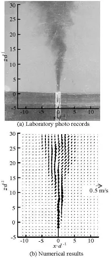
Fig.5 Comparison of jet instantaneous flow field in wave environment when the wave crest passes through the jet nozzle

The time-averaged vertical velocity distribution of the jet on the cross-section z/d=20 for Case W1 are plotted in Fig.3. The results of GSA show a narrower jet width compared with the experimental data，despite the reproduction of the “twin peaks”. However，with the grids getting finer， the difference between the numerical results gets smaller. Results of GSC and GSD are very close to each other， both are correlated well with the experimental data. The vertical profiles of the time-averaged velocity at three different downstream sections for Case C1 are shown in Fig.4. Among all numerical results， the results of GSA have the largest discrepancy with the experimental data. The difference between the numerical results of GSC and GSD is again quite small， and with the grid refinement，

the numerical results are closer to the experimental data， indicating that the numerical scheme is inherently convergent. Referring to the above results， the GSC grid system is fine enough for the simulation of the jet in either wave or cross-flow environments. Subsequently， the results of the grid system GSC are used to validate the model accuracy against the experimental data.

Fig.6 Time-averaged vertical velocity distribution of the jet in the wave environment （Case W1）

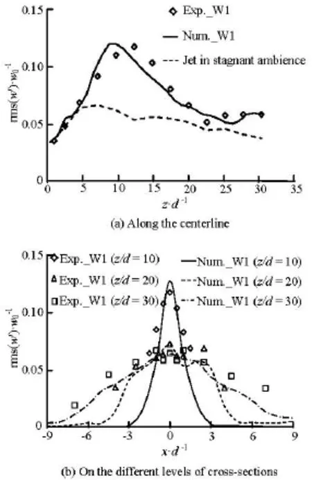
Fig.7 Velocity turbulence fluctuation rms（）w＇ of jet in the wave environment （Case W1）

Fig.8 Comparison of instantaneous flow field in cross-flow environment

3.2Model validation for the case of jet in wave environment

Figure 5 shows the qualitative comparison of the instantaneous jet flow in the wave environment （Case W1） when the wave crest passes through the jet nozzle. The jet body marked in Fig.5（b） is distinctly seen from the difference of the wave flow field with and without the existence of the jet. As shown in Fig.5（a）， the jet body sways to the right slightly due to the water particle velocity along the x direction in the laboratory experiments. This phenomenon is well reproduced by the numerical simulation， as shown in Fig.5（b）. Figure 6 shows the quantitative comparison of the time-averaged vertical velocity distribution. The good agreement between the numerical results and experimental measurements indicates that the current model can correctly reproduce the jet movement in the waveenvironment. According to the numerical results， the jet under the wave effect has a faster decay of the centerline velocity than that in the stagnant ambience， as shown in Fig.6（a）， and the “twin peaks” of the mean velocity exist in the cross-sectional profiles， as shown in Fig.6（b）. These findings are all consistent with the conclusions made by other investigators， such as Tam and Li［19］.

Fig.9 Comparison of vertical profiles of velocity magnitude on the symmetrical plane （=0）y between numerical results and experimental data at eight downstream sections of jet in cross-flow environment （Case C1）

Fig.10 Comparison of vertical profiles of velocity magnitude on the symmetrical plane （=0）y between numerical results and experimental data at five downstream sections of jet in cross-flow environment （Case C2）

Apart from the time-averaged velocities， the turbulent properties obtained from the numerical and experimental methods are also compared with each other. In order to separate the turbulence fluctuations from the fluctuations due to the wave effect， the jet turbulence fluctuations are calculated by using the instantaneous velocity values plus the phase-averaged velocity values. This method was illustrated in the papers of Mossa［6，7］when he experimentally studied the jet in the wave environment. Figure 7 shows the velocity turbulence fluctuation rms（）w＇ of the jet （a）along the centerline and （b） on the different levels of cross-sections. It can be seen from Fig.7 that the turbulence intensity of the jet in the wave environment is apparently larger than that in the stagnant ambience，indicating a mechanism of the enhanced jet mixing with the surrounding waters［6，7］. The maximum turbulence intensity occurs in the zone of deflection［4］，which shows that the interaction between the jet and the wave in this zone is the most significant. Further-more， the turbulence on the cross-sections gradually deviates from the Gaussian distribution， mainly due to the discontinuity of the jet centerline under the wavy motion［22］.

Fig.11 Velocity turbulence fluctuations rms（）u＇ and rms（）w＇ of jet in cross-flow environment （Case C1）

Fig.12 Velocity turbulence fluctuations rms（）u＇ and rms（）w＇ of jet in cross-flow environment （Case C2）

3.3Model validation for the case of jet in cross-flow environment

Figure 8 shows the qualitative comparison of the instantaneous jet flow in the cross-flow environment（Case C1）. Similarly， the jet body is distinctly seen from the difference of the cross-flow fields with and without the existence of the jet effect. The jet deflection along the cross-flow is clearly observed in both experimental and numerical studies.

Figure 9 shows the comparison of vertical profiles of the velocity magnitude on the symmetrical plane（=0）y between the numerical results and the experimental data at six downstream sections. The good agreement between simulation and experimental results indicates that the LES model can correctly simulate the jet near-field movement in the cross-flow environment. It is noted that there exists a node at the downstream location of /2xd≈， as shown in Fig.8， from where the flow field is separated into two regions， i.e.，the reverse and forward flow regions. This phenomenon was well described by Hsieh and Huang［1］.

Figure 10 shows the comparison of velocity magnitude profiles at three downstream sections （Case C2）. It can be seen that the numerical results generally agree well with the experimental data. Figure 10 also shows that only one maximum value is found on each section and the vertical position of this value gets higher at a further downstream location. However， two maximum values are observed on the same section of Case C1，as shown in Fig.9. The explanation of this phenomenon can be found in Fig.4. As the maximum horizontal and vertical velocity components do not reach the same height， it is understandable that the absolute velocity profiles may have two peaks.

Figure 11 shows the comparison of the velocity turbulence fluctuations rms（）u＇ and rms（）w＇ of the jet at six downstream sections （Case C1）. The model can reproduce the variation of the turbulence intensity along the water depth at each downstream section quite well. It can be seen that， with the jet moving downstream， the turbulent intensity gradually decreases， mainly because the jet's own momentum becomes weaker and weaker. The same findings are applicable in the case of C2， as shown in Fig.12.

3.4Model validation for the case of jet in wave and cross-flow coexisting environment

A comparative study is first carried out to investigate the accuracy of the modelling results using different inflow boundary conditions. As described above， NS1 represents the inflow conditions without the wave-current interaction， while NS2 represents the inflow conditions with the wave-current interaction. Figure 13 shows the comparison of the numerical re-sults using two different inflow boundary conditions for Case WC1， and Fig.14 for Case WC2. The corresponding experimental data are also plotted for comparison. The effects of the inflow boundary on the time-averaged vertical velocity profiles at several typical downstream sections are illustrated in Fig.13 and Fig.14. Generally， the agreement between the experimental data and the NS2 results is better than that between the experimental data and the NS1 results，especially at the section of /=0zd. When the interaction between the wave and the current is insignificant，e.g.， a strong cross-flow combined with a very small wave， the difference between the results of NS1 and NS2 could be neglected. However， when the interaction between the wave and the cross-flow becomes very strong， the results of NS1 may deviate from the real situation. Thus， the NS2 approach is recommended to generate the inflow boundary. The results shown below are based on the NS2 inflow boundary.

Fig.13 Comparison of experimental data and numerical results using two different inflow boundary conditions for Case WC1

Fig.14 Comparison of experimental data and numerical results using two different inflow boundary conditions for Case WC2

Fig.15 Comparison of instantaneous flow field of jet in wave and cross-flow coexisting environment when the wave crest passes through the jet nozzle

Fig.16 Jet instantaneous flow fields and streamlines in coexisting wave and cross-flow environment （Case WC1） on three different transverse planes at the wave crest phase

Figure 15 shows the physical photo record and the numerical instantaneous flow field of the jet in the wave and cross-flow coexisting environment （Case WC1） when the wave crest passes through the jet nozzle， in which the jet body is distinctly seen from the background flow using bold marks. The jet body is not only deflected along the cross-flow， but is also influenced significantly by the wave， which leads to the appearance of the “effluent clouds” on the upper partof the jet body. A similar phenomenon was found by Xia and Lam［23］when they studied a jet in an unsteady cross-flow environment. The position of the “effluent clouds” is well consistent with that shown in the photo. Figure 16 shows the jet instantaneous flow fields and streamlines on three different transverse planes on the wave crest phase. Plane 1 is located at the center of“effluent cloud” C1 （x/d=3）， Plane 3 is located at the center of “effluent cloud” C2 （x/d=12.1） and Plane 2 is located at the middle of “effluent cloud” C1 and “effluent cloud” C2 （x/d=7.5）. It can be seen that the flow structures on Plane 1 and Plane 3 are similar， while the flow structure on Plane 2 shows a different feature. Although the CVP structure can be seen on each plane， the vertical velocities above the CVP structure are significantly larger on Planes 1 and 3 than that on Plane 2， which indicates that the “effluent clouds” maintain part of the jet initial momentum and keep the jet body moving upwards inside the“effluent clouds”.

Fig.17 Comparison of vertical profiles of velocity magnitude on the symmetrical plane （=0）y between numerical results and experimental data of jet in wave and cross-flow coexisting environment （Case WC1）

Figure 17 shows the comparison of vertical profiles of the velocity magnitude on the symmetrical plane（=0）y between numerical results and experimental data at six downstream sections of the jet in the coexisting wave and cross-flow environment （WC1），which clearly shows good agreements between the numerical results and the experimental data.

Fig.18 Comparison of vertical profiles of velocity magnitude on the symmetrical plane （=0）y between numerical results and experimental data of jet in wave and crossflow coexisting environment （Case WC2）

Fig.19 Velocity turbulence fluctuations rms（）u＇ and rms（）w＇ of jet in wave and cross-flow coexisting environment （Case WC1）

Figure 18 shows the comparison of vertical profiles of the velocity magnitude on the symmetrical plane（=0）y between numerical results and experimental data at three downstream sections of the jet in the waveand cross-flow coexisting environment （Case WC2）. Again， the numerical results agree well with the experimental data， showing the general accuracy of the model under different conditions， which indicates that the model developed in this study can be generally used to simulate the jet movement in various wave and cross-flow environments.

Fig.20 Velocity turbulence fluctuations rms（）u＇ and rms（）w＇ of jet in wave and cross-flow coexisting environment （Case WC2）

Figure 19 and Fig.20 show the validation of the velocity turbulence fluctuations rms（）u＇ and rms（）w＇of the jet at downstream sections in Cases WC1 and WC2， respectively. It can be seen that the model gives an acceptable simulation of the turbulent normal stresses and correctly catches the peak values at each downstream section. In order to compare the turbulence properties of the jet in the wave and cross-flow environment and those in the cross-flow only environment， the velocity turbulence fluctuations rms（）u＇and rms（）w＇ of the jet in the cross-flow environment（Case C1） are drawn in Fig.19. As seen in Fig.19， at the downstream sections /=xd0， 2 and 4， the maximum turbulence intensities of the jet in the crossflow environment are higher than those in the wave and cross-flow environment， at the downstream sections /=xd7， 10 and 14， the maximum turbulence intensities of the jet in the wave and cross-flow environment become larger than those in the cross-flow only environment. Another apparent difference is that the turbulent normal stresses of the jet in the wave and cross-flow environment has a wider distribution than those of the jet in the cross-flow environment， which is strongly related to the existence of “effluent clouds”in the cases of the jet in the wave and cross-flow environment. In other words， the wave can have a positive effect on the mixing and diffusion of the jet in the wave and cross-flow environment.

4. Conclusion

A generic LES model is developed to simulate the jet movement in various wave and current environments. The model is well validated against experimental data in five representative cases， i.e. one case of the jet in the wave only environment， two cases of the jet in the cross-flow only environment and two cases of the jet in the wave and cross-flow coexisting environments. Numerical results show that， （1） the jet in the wave environment sways due to the wave effect，with a faster decay of the jet centerline velocity， a higher turbulence level and the appearance of “twin peaks” on the cross-sectional velocity profiles， （2） the jet in the cross-flow environment is deflected along the cross-flow with a node at the downstream， which leads to the separation of the flow field into reverse and forward flow regions， （3） the jet in the wave and crossflow coexisting environment is not only deflectedalong the cross-flow， but is also influenced significantly by the wave， which leads to the appearance of the“effluent clouds” on the upper part of the jet body and the enhancement of the mixing of the jet with surrounding waters. All results obtained are consistent with the experimental data， not only qualitatively but also quantitatively， showing that the model developed in this study is a generic tool to simulate the jet movement in various coastal environments.

References

［1］HSIEH R. H.， HUANG R. F. Tomographic flow structures of a round jet in a crossflow［J］. Journal of China Industrial Engineering， 2003， 26（1）: 71-80.

［2］YUAN L. L.， STREET R. L. and FERZIGER J. H. Largeeddy simulations of a round jet in crossflow［J］. Journal of Fluid Mechanics， 1999， 379: 71-104.

［3］CAMBONIE T.， GAUTIER N. and AIDER J. L. Experimental study of counter-rotating vortex pair trajectories induced by a round jet in cross-flow at low velocity ratios［J］. Experiments in Fluids， 2013， 54（3）: 1475-1497.

［4］CHYAN J. M.， HWUNG H. H. On the interaction of a turbulent jet with waves［J］. Journal of Hydraulic Research， 1993， 31（6）: 791-810.

［5］SHARP D. B.， SHAWCROSS A. and GREATED C. A. LIF measurement of the diluting effect of surface waves on turbulent buoyant plumes［J］. Journal of Flow Control，Measurement and Visualization， 2014， 2（3）: 77-93.

［6］MOSSA M. Experimental study on the interaction of nonbuoyant jets and waves［J］. Journal of Hydraulic Research， 2004， 42（1）: 13-28.

［7］MOSSA M. Behavior of nonbuoyant jets in wave environment［J］. Journal of Hydraulic Engineering， ASCE，2004， 130（7）: 704-717.

［8］HSIAO S. C.， HSU T. W. and LIN J. F. et al. Mean and turbulence properties of a neutrally buoyant round jet in a wave environment［J］. Journal of Waterway， Port， Coastal， and Ocean Engineering， 2011， 137（3）: 109-122.

［9］CAVAR D.， MEYER K. E. LES of turbulent jet in crossflow: Part 1-A numerical validation study［J］. International Journal of Heat and Fluid Flow， 2012， 36: 18-34.

［10］ CAVAR D.， MEYER K. E. LES of turbulent jet in crossflow: Part 2-POD analysis and identification of coherent structures［J］. International Journal of Heat and Fluid Flow， 2012， 36: 35-46.

［11］ CHEN Y. P.， LI C. W. and ZHANG C. K. Numerical modeling of a round jet discharged into random waves［J］. Ocean Engineering， 2008， 35（1）: 77-89.

［12］ LU Jun， WANG Ling-ling and TANG Hong-wu et al. Numerical investifation of vertical turbulent jets in different types of waves［J］. China Ocean Engineering， 2010，24（4）: 611-626.

［13］ MULDOON F.， ACHARYA S. Direct numerical simulation of pulsed jets-in-crossflow［J］. Computers and Fluids，2010， 39（10）: 1745-1773.

［14］ ZHANG Hui， YANG Jian-min and XIAO Long-fei et al. Large-eddy simulation of the flow past both finite and infinite circular cylinders at Re=3900［J］. Journal of Hydrodynamics， 2015， 27（2）: 195-203.

［15］ LIN P.， LI C. W. A -σcoordinate three-dimensional numerical model for surface wave propagation［J］. International Journal of Numerical Methods Fluids， 2002，38（11）: 1045-1068.

［16］ YOU Z. J. The effect of wave-induced stress on current profiles［J］. Ocean Engineering， 1996， 23（7）: 619-628.

［17］ PARK J. K.， KIM M. H. and MIYATA H. Three-dimensional numerical wave tank simulations on fully nonlinear wave-current-body interactions［J］. Journal of Marine Science and Technology， 2001， 6（2）: 70-82.

［18］ CHEN Yong-ping， LI Chi-Wei and ZHANG Chang-kuan. Large eddy simulation of vertical jet impingement with a free surface［J］. Journal of Hydrodynamics， Ser. B， 2006，18（2）: 148-155.

［19］ TAM B. F.， LI C. W. Flow induced by a turbulent jet under random waves［J］. Journal of Hydraulic Research，2008， 46（6）: 820-829.

［20］ LEE J. H. W.， KUANG Cui-ping and CHEN Guo-qian. The structure of a turbulent jet in a crossflow: Effect of jet-crossflow velocity［J］. China Ocean Engineering，2002， 16（1）: 1-20.

［21］ ZHOU X.， LUO K. H. and WILLIAMS J. J. R. Largeeddy simulation of a turbulent forced plume［J］. European Journal of Mechanics- B/Fluids， 2001， 20（2）: 233-254.

［22］ XU Z.， CHEN Y. and ZHANG C. et al. Comparative study of a vertical round jet in regular and random waves［J］. Ocean Engineering， 2014， 90: 200-210.

［23］ XIA L. P.， LAM K. M. Unsteady effluent dispersion in a round jet interacting with an oscillating cross-flow［J］. Journal of Hydraulic Engineering， ASCE， 2004， 130（7）: 667-677.

（February 7， 2015， Revised November 11， 2015）

* Project supported by the National Natural Science Foundation of China （Grant Nos. 51379072， 51109074）， the Specialized Research Fund for the Doctoral Program of Higher Education （Grant No. 20120094110016）， the 111 Project of the Ministry of Education and the State Administration of Foreign Experts Affairs， China （Grant No. B12032） and the Fundamental Research Funds for the Central Universities （Grant No. 2014B02514）.

Biography： Zhen-shan XU （1988-）， Male， Ph. D.， Lecturer

Yong-ping CHEN，

E-mail: ypchen@hhu.edu.cn