Experimental research on seismoelectric effects in sandstone*

Peng Rong, Wei Jian-Xing, Di Bang-Rang, Ding Pin-Bo♦, and Liu Zi-Chun

Experimental research on seismoelectric effects in sandstone*

Peng Rong1,2,3, Wei Jian-Xing1,2,3, Di Bang-Rang1,2,3, Ding Pin-Bo♦1,2,3, and Liu Zi-Chun1,2,3

The seismoelectric effects induced from the coupling of the seismic wave field and the electromagnetic field depend on the physical properties of the reservoir rocks. We built an experimental apparatus to measure the seismoelectric effects in saturated sandstone samples. We recorded the seismoelectric signals induced by P-waves and studied the attenuation of the seismoelectric signals induced at the sandstone interface. The analysis of the seismoelectric effects suggests that the minimization of the potential difference between the reference potential and the baseline potential of the seismoelectric disturbance area is critical to the accuracy of the seismoelectric measurements and greatly improves the detectability of the seismoelectric signals. The experimental results confirmed that the seismoelectric coupling of the seismic wave field and the electromagnetic field is induced when seismic wave propagating in a fluid-saturated porous medium. The amplitudes of the seismoelectric signals decrease linearly with increasing distance between the source and the interface, and decay exponentially with increasing distance between the receiver and the interface. The seismoelectric response of sandstone samples with different permeabilities suggests that the seismoelectric response is directly related to permeability, which should help obtaining the permeability of reservoirs in the future.

Seismoelectric effects, seismoelectric response, potential difference, sandstone, permeability

Introduction

Seismoelectric signals are generated by the interaction of seismic and electromagnetic waves in fluid-filled porous media. The seismoelectric signals depend on the physical parameters of the reservoirs, such as permeability, porosity, fluid, seismic wave velocity, etc. Therefore, they can be used in reservoir description.

Pride (1994) and Haartsen and Pride (1996) proposed the seismoelectric conversion model in porous media by introducing the seismoelectric coupling coefficient, but the model is only suitable for saturated porous media. Revil et al. (2015) extended the seismoelectric conversion model to partially saturated porous media: including two cases, one is the nonwetting phase (air)in porous medium at atmospheric pressure; the other is two immiscible Newtonian pore fluids in pore space. Zhu et al. (1994, 2015) and Zhu and Toksöz (2005) performed series of seismoelectric measurements on a layered model, a borehole model, and a rock sample and observed the interface response field and the coseismic field. Block and Harris (2006) simulated the seismoelectric phenomena in fluid-saturated sediments and studied the conductivity dependence of the seismoelectric effects by changing the fluid composition. Shakel et al. (2011b, 2011c) carried out experimental and theoretical work on the seismoelectric response in a small-scale rock model immersed in water. Pengra et al. (1999) measured the electroosmotic pressure and streaming potential of natural and artificial samples to obtain the permeability of the latter. The experimental work on seismoelectric effects and reservoir parameters improved our understanding of seismoelectric conversion. Deckman et al. (2005) conducted electrokinetic experiments on different rock samples, which were saturated at various fluid concentrations, and analyzed the relation between the seismoelectric coupling coefficient, solution concentration, and pore size. Key reservoir parameters, such as permeability, porosity, and zeta potential and the relation between pore size and seismoelectric signal were obtained by experimenting with the streaming potential (Dukhin et al., 2010; Dukhin and Shilov, 2010; Wang et al., 2015a). Glover (2012a; 2012b) examined the dependency of the streaming potential on frequency and described the streaming potential coefficient as a function of frequency. Zhu et al. (1994) and Zhu and Toksöz (2005) carried out seismoelectric measurements on a layered borehole model and a fractured borehole model; moreover, Zhu and Toksöz (2003) completed crosshole seismoelectric measurements under transient or highfrequency excitation. Zhu and Toksöz (2012) studied multipole seismoelectric logging while drilling (LWD) and found that the method can be used to retrieve the formation velocity without the effect of tool waves. Wang et al. (2015a, 2015b) obtained the P- and S-wave velocities of sandstone by using seismoelectric logging while drilling. Surkov et al. (2002) investigated the effect of the possible fractal structure in the earthquake hypocenter zone on seismoelectric phenomena. A fault induces an earthquake and wavefields are assumed to be generated by the slip of small faults and to be equivalent to those generated by a double-couple source. The seismoelectromagnetic field induced by series of small faults were numerically modeled to study the electromagnetic disturbance of the fault rupture (Gao and Hu, 2010; Hu and Gao, 2011). Gershenzon et al. (2014) studied the coseismic electromagnetic field owing to the electrokinetic effect and the results were used to explain the electric and magnetic disturbances caused by an earthquake and for studying the earth’s upper crust.

The magnitude of the seismoelectric signal in rocks is in the range of a few dozen microvolts to hundreds of microvolts, and it is difficult to detect because it is easily affected by the surrounding noise. Zhu et al. (1999) showed that the seismoelectric signal is the voltage between electrodes and ground using borehole models. The seismoelectric effects in sand saturated with multiphase fluid has been measured with two electrodes; one electrode was used to obtain the potential disturbance of the seismoelectric conversion and the other distal electrode to obtain the reference potential (Chen and Mu, 2005). In studying seismoelectric phenomena in fluidsaturated sediments with a cylindrical tube apparatus, the apparatus was placed inside a copper-mesh cage to protect it from electrical interference. The coppermesh cage also grounded the entire apparatus (Block and Harris, 2006). Schakel et al. (2011a) and Smeulders et al. (2014) studied the electrode data relative to the grounding using rock samples immersed in a water tank. Filtering and multiple stacking were adopted in these experiments to suppress the interference and reduce the random noise.

Based on past work and because seismoelectric measurements were performed without shielding, the acquisition of seismoelectric signals has high uncertainty and instability, we built up a seismoelectric apparatus without shielding to overcome the above-mentioned problems. The seismoelectric measurements suggest that the minimization of the potential difference between the reference potential and the ground potential of the signal in the disturbed area can greatly improve the detectability and stability of the seismoelectric measurements. We measured the seismoelectric conversion in saturated sandstone samples. The seismoelectric signals depend on the permeability variation and may provide a credible basis for the identification of reservoir fluids.

Generation of the seismoelectric effects

A seismic wave traveling through a fluid-filled porous material creates fluid pressure gradients and grain acceleration that induce pore fluid flow. The disturbance in the electrical double layer (Shaw, 1992) causes relative motion between the movable charges in the pore fluidand the fixed charges on adjacent grains. The net flow of charges creates an electric field. This field represents a seismoelectric effect of the second type that can generate two kinds of seismoelectric field, the coseismic field, and the seismoelectric interface response field.

The coseismic field is induced in homogeneous media (Figure 1), where the diffuse-layer ions accumulate in the peaks and troughs of the P-wave, creating electric fields that are perpendicular to the wavefront and drive conduction currents. In a homogeneous medium, the conduction current exactly balances the streaming current; therefore, the total current is zero and there are no magnetic fields. Independently propagating EM waves are not generated. There is an electric field moving along with the P-wave (Haartsen and Pride, 1997). The formation of an electric double layer is related to the composition of the medium particles and reservoir properties; hence, the coseismic field gives information for the area around the receiving electrodes. On the seismoelectric record, this field travels along with the seismic wave and only when the seismic wave produces disturbances around the electrodes, the electrodes detect the coseismic signals. The apparent velocity of the coseismic field equals the wave velocity in the formation and the arriving time of the coseismic signal is related to the distance between the electrodes and the source.

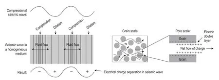
Fig.1 First-kind electric field owing to the second-kind seismoelectric effect: the coseismic field is induced by the propagation of the P-wave (Pride, 1994).

In an inhomogeneous medium, when a seismic wave encounters a layer with different properties (electrical, flow-related, and petrophysical), the charge balance is disturbed and an electromagnetic field is created (Figure 2). This electromagnetic field is the seismoelectric interface response field, which can be described as an electric dipole perpendicular to the interface, oscillating with the change of the seismic waveform and forming at the first Fresnel zone (Thompson and Gist, 1993; Haartsen and Pride, 1997). At seismic frequencies, the interface response field is typically regarded as the electric field generated by quasi-static electric dipoles (Garambois and Dietrich, 2001). Compared to the traveltime of the seismic wave from the source to the interface, the traveltime of the interface response field propagating from the interface to the receiving electrode is negligibly smallTherefore, the change in the distance between the electrodes and the seismic source does not affect the traveltime of the interface response. As long as the distance between the source and the interface does not change, the interface response arrives at each electrode simultaneously. The seimoelectric interface response field provides information about the interfaces below the surface. In particular, thin-layered structures, such as fracture zones, permeability zones, and thin reservoirs, can produce strong seismoelectric interface responses.

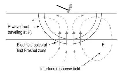
Fig.2 Second-kind electric field owing to the secondkind seismoelectric effect: the interface response field is induced at the interface of media with different properties (Haines et al., 2007).

Seismoelectric measurements

Experimental setup

A P-wave transducer was used to simulate the source. The generated P-wave propagated in the fluid-filled rock sample and induced seismoelectric coupling. The induced seismoelectric signals were received by an electrode and seismoelectric responses were generated at the rock samples with different physical properties. Figure 3 shows the experimental setup for measuring the seismoelectric effects. The rock, the electrode, and the transducer are inside a Plexiglas tank. The distance between the three is adjustable and the 200 cm × 150 cm × 100 cm tank is filled with tap water. The 300 V ultrasonic pulse transducer (model 5077PR) sends an electric impulse to the 500 kHz P-wave transducer and a low-amplitude trigger to the oscilloscope. The P-wave travels in the water, reaches the sandstone rock sample, and induces seismoelectric coupling by the wave pressure gradient. The seismoelectric signal is received by a 0.5 mm diameter electrode (Ag/AgCl) and is amplified by a preamplifier with 60db gain (Olympus ultrasonic preamplifier 5660c) and transferred to the oscilloscope (Agilent Technology DSO6012A). The oscilloscope records the seismoelectric signals once it is triggered. The electrode potential is given relative to the common ground. The vertical and the horizontal resolution of the oscilloscope are adjusted to 20 mv/ grid and 10 us/grid, respectively. The stacking times of the signal are set to 1024, and the resolution and superposition times guarantee that the signal is detectedby the oscilloscope. A computer is used for the signal acquisition and data processing.

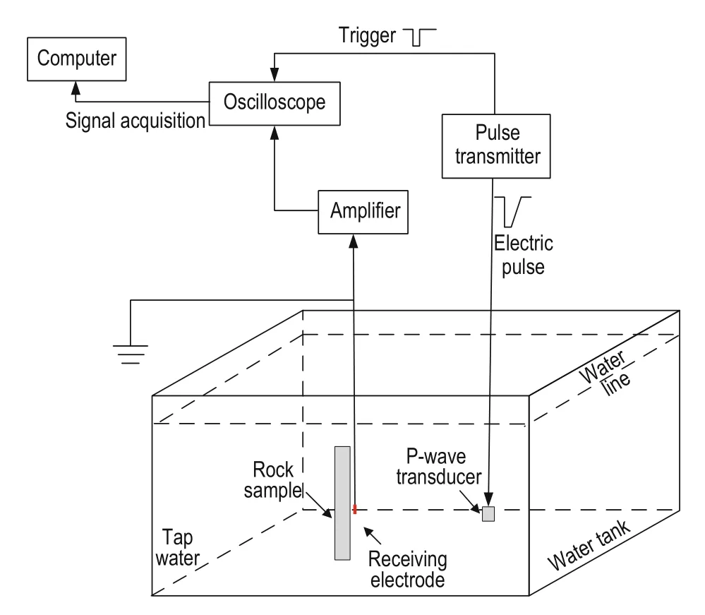
Fig.3 Schematic of the experimental setup for measuring the seismoelectric effects.

Two methods were used in the seismoelectric experiment (Figure 4). d1 is the distance between the acoustic source and the sandstone interface, d2 is the distance between the electrode and the sandstone sample. In the first method, the acoustic source is moved at 1 cm/trace to change d1 while the electrode is set at the sandstone interface (d2 = 0). The second method is changing d2 by moving the electrode at 0.5 cm intervals and keeping the d1 unchanged. The signal acquisition starts when d2 = 0. The seismoelectric signal is recorded with every movement of the electrode.

Fig.4 Schematic of the two methods for making seismoelectric measurements: (1) moving the acoustic source to change d1 with the electrode set at the sandstone interface; (2) changing d2 by moving the electrode at 0.5 cm intervals and keeping d1 unchanged.

The measuring principle of seismoelectric signal

The apparatus (Figure 3) was designed to measure the weak seismoelectric signal generated in the rock sample. The weak seismoelectric signal is first amplified. Then, to avoid signal distortion, the signal goes to the amplifier without being filtered and the seismoelectric measurementis taken in the stage from the receiver to the first amplifier.

The front panel of the preamplifier used in the experiment is shown in Figure 5a. The preamplifier is based on the difference principle, in which the signal is enhanced by the voltage difference in the two input voltages. When the measured signals are separately obtained from two different points and the voltage difference between the two points is represented as a value, the measured signal is called the differential signal. In some cases, the “ground” is the reference pointfor the measured signal and the voltage of the single point represents the measured signal that is transmitted by one wire. This type of signal is called single-end signal and is a special differential signal. As shown in Figure 5b, the input to the amplifier has only one port (the positive input) and the reference voltage (the negative input) is equipotential with the "ground" as well as the potential of the shielding of the signal cable. The seismoelectric signal received by the amplifier is the potential difference (ΔVout) between the signal received by the electrode and the "ground".

The seismoelectric signal is transferred from the electrode to the amplifier as single-end input. The ground potential of two points should be close to each other when using the single-end input to transmit a signal from one point to the other. If the ground potential difference between the electrode and the amplifier exceeds a certain range, which is related to the relative amplitude of the measured signal, the amplifier fails to detect the useful signal. In general, when the potential of the reference point is sufficiently steady, the higher potential difference between the reference point and the measurement point is easily detected.

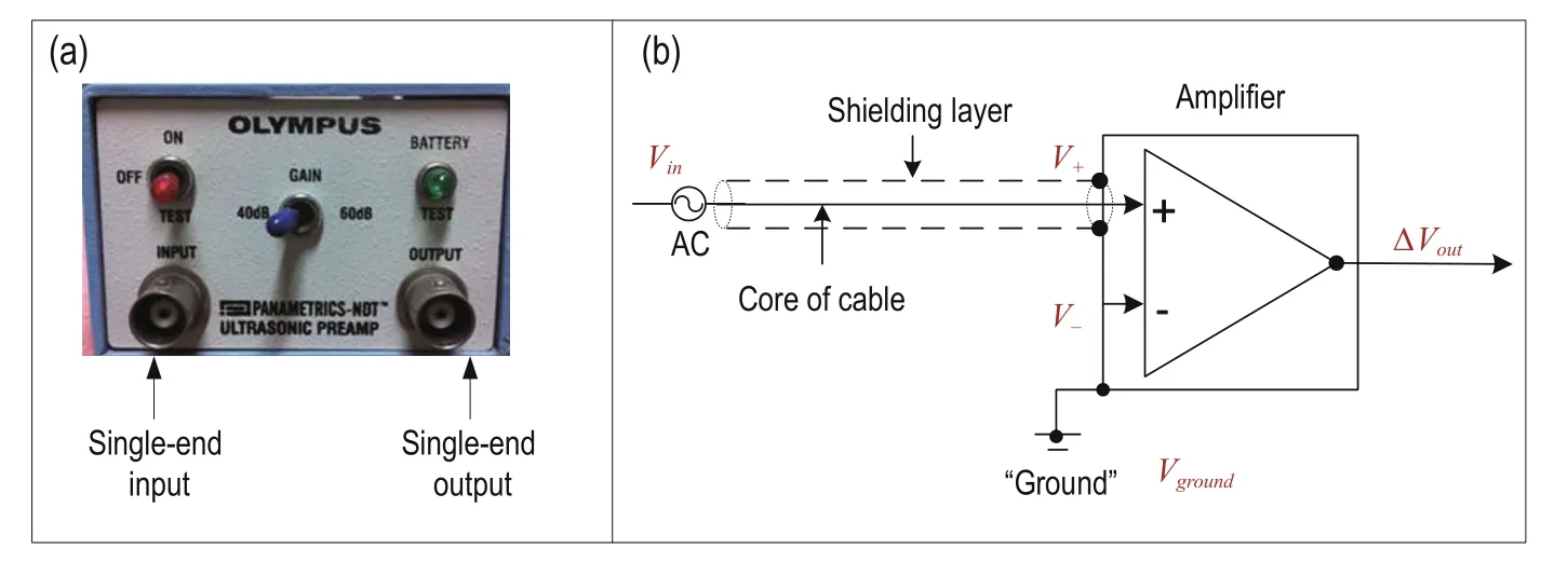
Fig.5 Front panel of the amplifier (a) and simplified diagram for the single-end input to the amplifier (b).

Figure 6 shows the schematic for the signal transmission between the receiving electrode and the amplifier. The input to the amplifier (positive input) Vincomprises the "ground" potential of the signal source Vground1and the seismoelectric disturbance VSE. The negative input V–is the ground potential Vgroundand ΔVoutis the output signal.

The measuring principle of the seismoelectric signal is described with following equations

Fig.6 Schematic of the signal transmission between the receiving electrode and the amplifier.

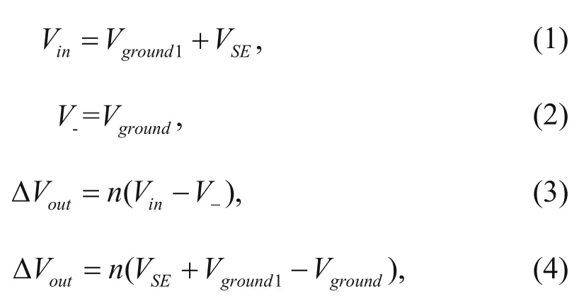
where Vinis the input signal of the electrode, Vground1is the "ground" potential of the signal source, VSEis the seismoelectric disturbance, V–is the potential of the reference point, V–equals the ground potential Vground, ΔVoutis the output signal after amplification, n is the magnification, and Vground1– Vgroundis the ground potential difference.

From these equations, it is found that when Vground1– Vgroundis not small (assumed 1 V)—a VSEequal to 10 V can be identified by the amplifier—the 1 V ground potential difference introduces errors and does not affect the signal recognition. However, the seismoelectric disturbance VSEis weak with magnitude of tens of microvolts to hundreds of microvolts, which is very small relative to the ground potential difference of 1 V. Therefore, the amplifier only detects the ground potential difference ΔVout≈ n(Vground1– Vground) and the small seismoelectric disturbance is ignored. Therefore,the identification of the seismoelectric signal depends on the consistency of the "ground" between two points.

Let us consider the seismoelectric experiment in the water tank, for example. We decreased the ground potential difference to acquire the seismoelectric signal. The first grounding method is shown in Figure 7a. The computer, oscilloscope, and pulse transmitter were connected to the same “ground” to make the potential of the instruments equal to the common ground potential (yellow line). In addition, a wire was attached to the“ground” with one end in the water to ensure that the potential of the water tank is the same as the common ground potential. The entire system is connected to the same “ground”, the reference potential is connected to an infinite potential—the grounding line of the amplifier is the input of the reference potential and the ground potential can be regarded as infinite potential. Therefore, the potential difference between the measured signal and the reference signal was sufficiently large; nevertheless, no seismoelectric signal was observed.

The second grounding method (Figure 7b) was used to improve the grounding conditions. The BNC shell of the amplifier input is directly connected to the common ground wire with a high-conductivity wire. The BNC shell of the amplifier input is connected with the shielding wire of the electrode and the common ground of the amplifier’s internal circuit. The connection of the wire is used to directly ground the shielding wire of the electrode, reducing the grounding resistance caused by the amplifier enclosure. However, we did not detect the seismoelectric signals.

The third grounding method is shown in Figure 7c. A high-conductivity wire was used, with one end connected to the BNC shell of the amplifier input and the other end placed in the water tank near the rock sample, which ensures that the reference voltage Vgroundof the amplifier input is consistent with the ground potential Vground1of the seismoelectric source. The wire connecting the amplifier and the “ground” of the instruments was removed, which increased the electromagnetic interference to the circuit of the amplifier and electrode, because the“ground” of the instruments was not the “ground” ofthe seismoelectric disturbance. However, seismoelectric coupling was not detected with this kind of grounding method.

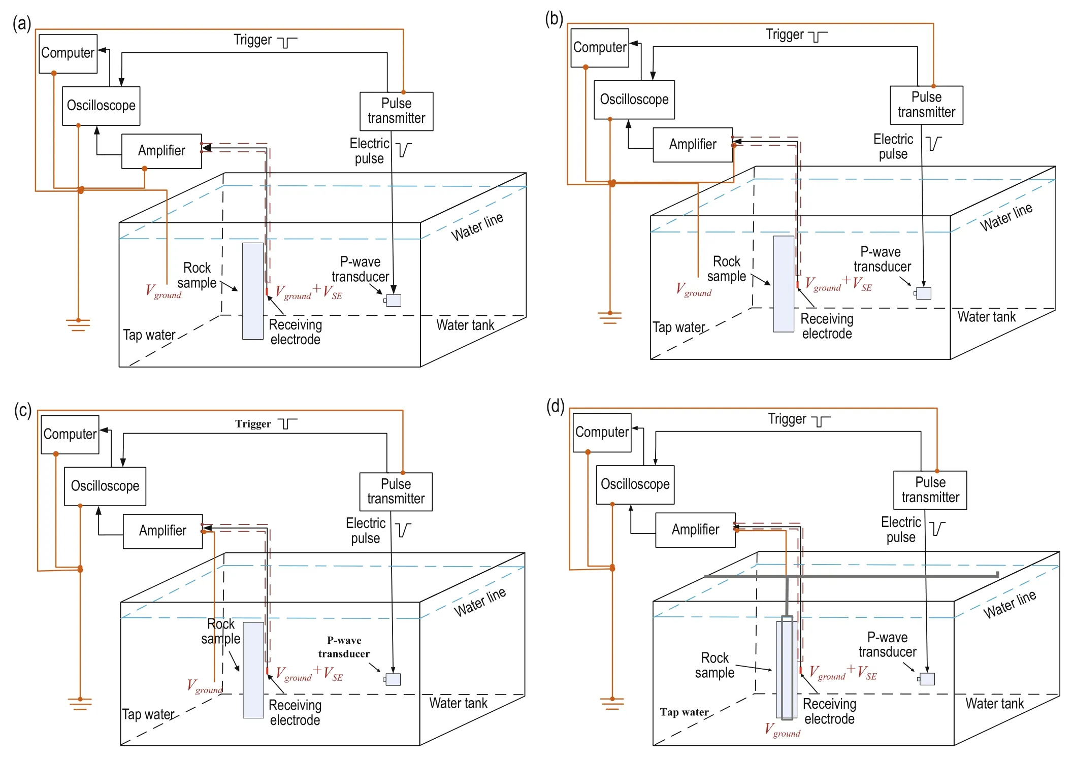
Fig.7 Grounding of the seismoelectric measuring system: (a) first grounding method, (b) second grounding method, (c) third grounding method, and (d) forth grounding method.

Actually, a wire connected to water cannot ensure that the potential of the entire water tank is the same as that of the common ground because the water resistance is high. In addition, the common ground is not the“ground” of the seismoelectric signal source and there is no correlation between the two “grounds”, which means that the “ground” potential between the reference point and the electrode has great potential difference. Hence, the amplifier cannot recognize the seismoelectric disturbance.

The consistency between the "ground" potential Vground1of seismoelectric signal source and the reference potential Vgroundof amplifier input was taken into consideration in the third grounding method but the reference potential Vgroundin the wire was not stable. Various factors would cause the variability of the reference potential, such as the electromagnetic interference of the surroundings, the oscillation of the water, etc. When the other end of the connecting wire was placed at different locations in the water tank near the rock sample, varying degrees of baseline drift appeared (Figure 8) because of the bad grounding. The baseline drift affected the ability of the amplifier to detect the seismoelectric disturbance. In Figure 8, it is seen that the potential drift changes as the positions of the other end of the connecting wire change. The zero baseline voltage suggests that no baseline drift is produced. The potential drift denoted by the red line is the minimum as well as the jitter of the signal voltage; this signal was obtained when the other end of the connecting wire touched the metal stent, which is used for fixing the rock sample.

According to the results of the third grounding method, the fourth grounding mode was used to ensurethe stability of the reference potential. A larger metal frame was used as the rock sample holder to stabilize the reference potential (Figure 7d). The wire with one end connected to the BNC shell of the amplifier input was indirectly connected with the rock sample through the metal frame. The latter has good conductivity and the contact area between the metal frame and the rock sample is large. The seismoelectric signal was obtained with this grounding method.

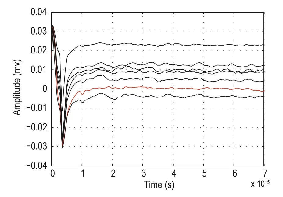
Fig.8 Baseline drift with the connecting wire placed at different position in the water tank in the third grounding method.

In the fourth grounding mode, the wire was connected with the metal frame, the metal frame was connected with the rock sample, and the electrode was close to the rock sample. Hence, the reference potential is equipotential with the ground potential of the electrode through the connecting wire. The sensitivity of the metal frame to potential changes is lower than that of the end of the single wire, and the “ground” formed by the metal frame is stable. Therefore, the amplifier can identify the seismoelectric signals because of the consistency and the stability of the ground potential.

The schematic of the signal transmission between the electrode and amplifier after grounding is shown in Figure 9. The wire connected to the BNC shell of the amplifier input with the metal frame ensures that the ground potential of the signal source Vground1equals the reference potential Vgroundby connecting the two potentials to a common virtual ground. Equation (4) is then expressed as

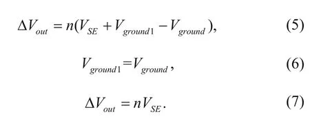
Hence, the signal that is eventually identifiedand amplified by the amplifier is the seismoelectric disturbance VSE. The two points, keeping the ground potential difference between the disturbed zone of the seismoelectric conversion and the input of the amplifier as small as possible and ensuring the stability of the ground potential, are critical to the seismoelectric measurements. The above-described measuring principle is widely applicable.

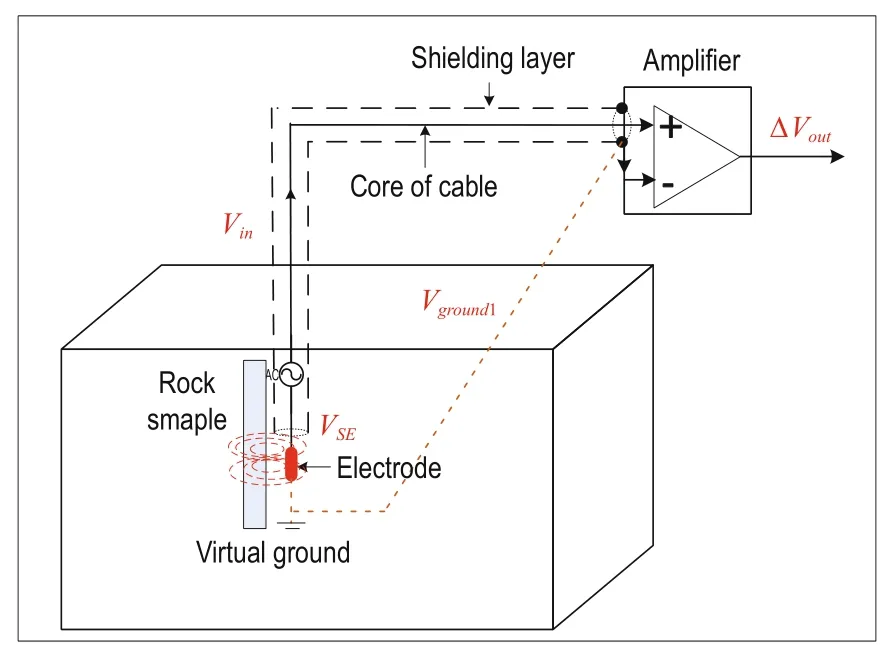
Fig.9 Schematic of the signal transmission between the receiving electrode and the amplifier after grounding.

In the seismoelectric signal acquisition, we tried to use different electrical equipment around the seismoelectric measurement setup. We found that the correct implementation of the two key points ensures the detection of the seismoelectric signal. The interference of the electrical equipment around the seismoelectric measurement system will not affect the detection of the seismoelectric signal, only the signal-to-noise ratio of the seismoelectric measurement. Therefore, clear and stable seismoelectric signals can be obtained without a shielded chamber.

Results

We recorded the seismoelectric signals in the saturated sandstone by using the fourth grounding mode. The schematic of the setup is the same as that in Figure 4. The dimensions of the rock sample were 10 cm × 10 cm × 5 cm and the excitation voltage was 400 V. The gain of the amplifier was set at 60 dB. The physical parameters of the rock samples are given in Table 1. The values for εsand εfare taken from the literature (see below). The values for ρ, Ø, k, and λ were measured directly.

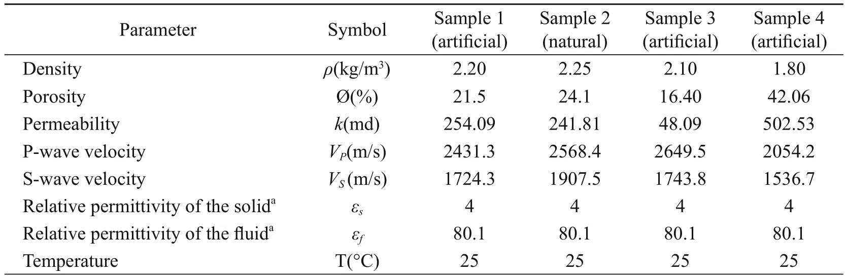
Table 1 Physical properties of the water-saturated rock sample

Confirmation of the seismoelectric conversion

To confirm that the measured signal is due to the seismoelectric conversion in the sandstone sample, we conducted a control experiment by using rock sample 1. We collected the signal with or without sample and with or without an acoustic wave source, respectively. During the measurements, the electrode was set at the rock sample and the distance between the acoustic source and the rock sample was about 9 cm. Figure 10 shows the results of the control experiment. Trace 0 was the acoustic signal and appeared at approximately 62 μs. Trace 1 was collected when the sandstone sample was placed on a clamp holder and the P-wave transducer was powered off (no wave source). We can see that trace 1 was almost horizontal with no disturbance. This indicates that the noise generated by the electrical equipment cannot induce seismoelectrical signals in the rock sample. Trace 2 was measured when there is no sample in the clamping bracket and the P-wave transducer was excited. From the results, we see that an electric pulse appears at time zero, and some small disturbances exist but no clear electrical signals appear near the time of the P-wave signal. This suggests that the high-voltage electrical pulse at the start is caused by the acoustic source. When the electric pulse drives the P-wave transducer to generate the acoustic wave, a high-voltage electric pulse induces electrical signals in the electrode. The high-voltage electric pulse cannot be eliminated by shielding or grounding. This high-voltage electric pulse does not exist in the seismic recordings; therefore, the high-voltage electric pulse also means that seismoelectrical signals are identified. As there is no sample in the water tank in trace 2, no seismoelectrical signals were detected. The small disturbances are background noise owing to the excitation of the acoustic source. Trace 3 is the signal obtained in the case of the sandstone sample placed in the clamp holder (with rock sample) and the P-wave transducer was powered on (with wave source). From trace 3, we can see a clear waveform appeared at 62 μs, which is equal to the traveltime of the P-wave from the source to the rock sample in water—the velocity of the acoustic wave in water is about 1480 m/s. This indicates that the signal received by the electrode is the seismoelectric conversion induced by the propagation of the P-wave in the rock sample.

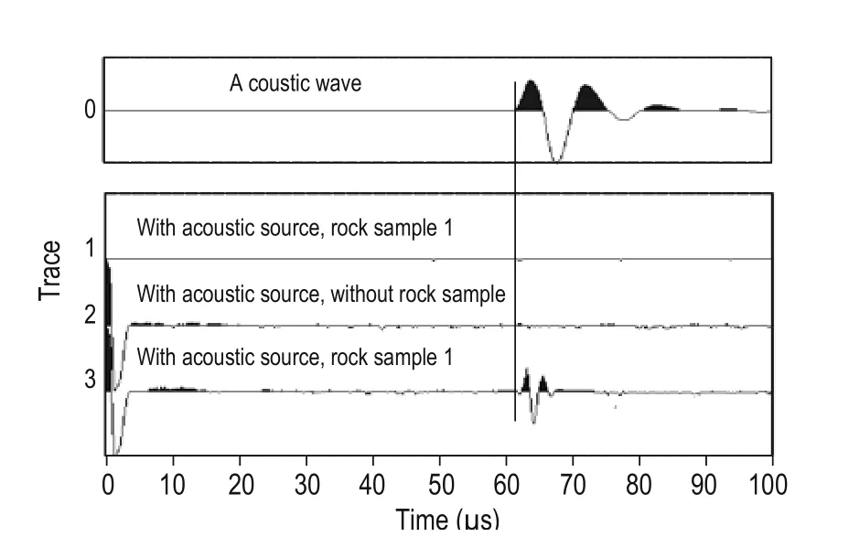
Fig.10 Results of the control experiment.

Seismoelectric response at the sandstone interface

We performed seismoelectric measurements on rock sample 1 by using the first and second measuring method in Figure 4. Figure 11 shows the seismoelectric signals recorded in the first measuring method. In Figure 11a, high-voltage electrical pulses are present at the start. The amplitude of the seismoelectric signal in trace 1 is the largest and decreases with increasing distance between the acoustic source and the sandstone interface. The velocity of the acoustic wave in water is about 1480 m/s. When d1 = 5 cm, the traveltime for the acoustic wave propagating from the source to the sandstone interface is about 33 μs and the seismoelectric pulse for trace also appeared at 33 μs for trace 1. The arrival time of the seismoelectric signals increases with increasing the distance between the acoustic source and the sandstone interface. The traveltime of the seismoelectric signals equals the one-way traveltime of the acoustic wave from the source to the sandstone based on the calculation of the arrival time of each seismoelectric signal. The results suggest that seimoelectric conversion is induced only when the acoustic wave reaches the rock. The measured seismoelectric signals are attributed to the seismoelectric interface response field of the second-kind seismoelectric effects.

Figure 11b shows the amplitude attenuation of the seismoelectric signal with increasing distance of the acoustic source from the interface. The comparison of the measured signal (star point) and the fitted line (inclined line) shows that amplitude of the induced seismoelectric signal is linearly attenuated with increasing distance of the acoustic source from the interface. Because the source spacing varies, the energy of the acoustic signal arriving at the interface decreases with increasing spacing. If observed closely, the linear increase in the source spacing leads to linear decreases in the P-wave energy; moreover, the seismoelectric signals induced by the P-wave decrease linearly.

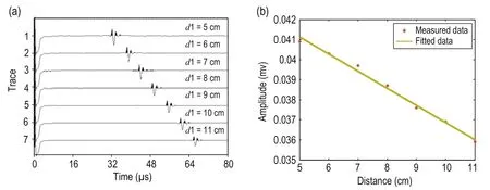
Fig.11 (a) Seismoelectric signals obtained by using the first measuring method. (b) Attenuation of the seismoelectric signal with increasing distance between the acoustic source and the interface.

The experimental results obtained with the second measuring method are shown in Figure 12a. The amplitude of the seismoelectric signal for trace 1 (the electrode was set at the interface) is larger than that of the other traces. The amplitude of the signal decays rapidly as the distance of electrode and interface (d2) increases but the time of the appearance of the electrical signal is the same and equal to the one-way traveltime of the acoustic wave propagating from the source to interface; the traveltime of the seismoelectric signals from the interface to the electrode is almost zero. These phenomena confirmed that the measured signal was the seismoelectric signal of the interface response field, because the interface response signal propagated athigh velocity (several orders of magnitude higher than the acoustic wave velocity), and the traveltime for the seismoelectric signals from the interface to the electrode could be ignored.

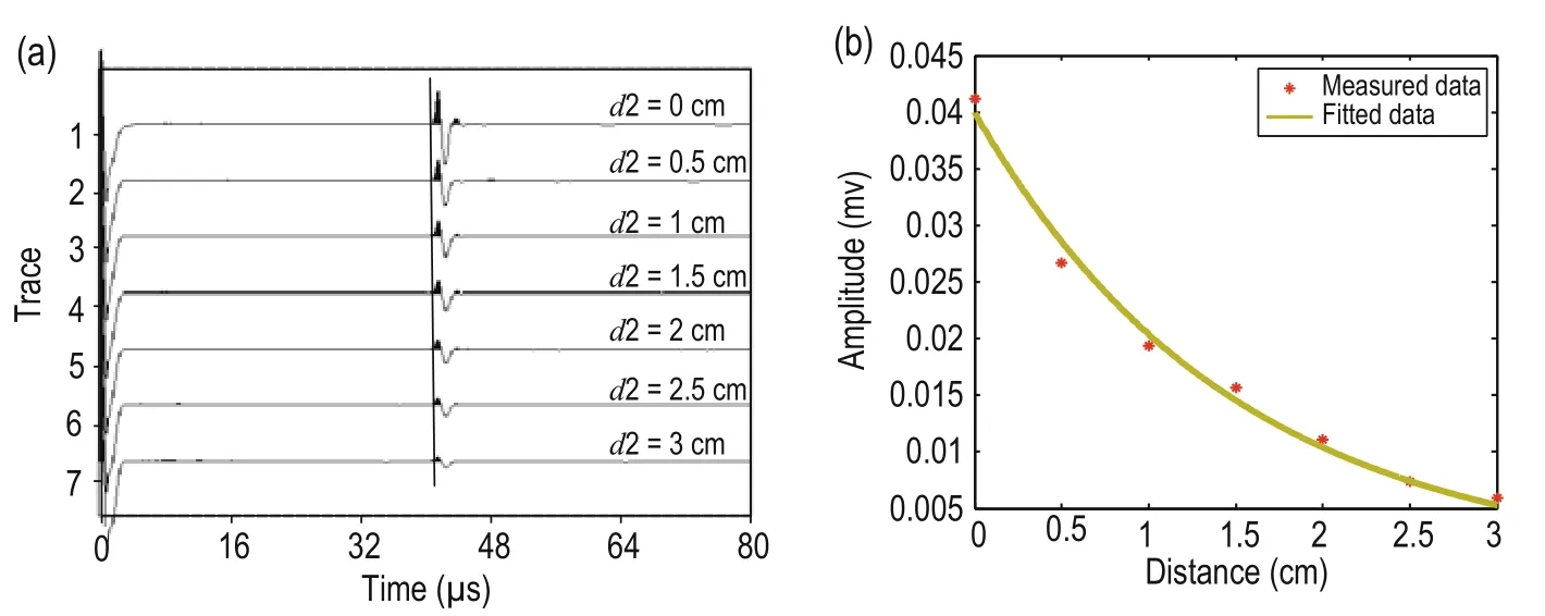
Fig.12 (a) Seismoelectric signals obtained by the second measuring method. (b) Attenuation of the seismoelectric signal with increasing distance between the electrode and the interface.

The amplitude of the seismoelectric signal decays exponentially with increasing distance between the electrode and the interface (Figure 12b). The results in Figures 11b and 12b suggest that when the distance between the acoustic source and the sandstone interface remains unchanged and the distance between the electrode and sandstone interface increases, the energy of the seismoelectric signal attenuates rapidly. When the distance of the electrode and sandstone interface remains unchanged and the distance of the acoustic source and sandstone interface increases, the amplitude of the seismoelectric signal decays slowly. Therefore, the energy loss of the seismoelectric signal caused by the increasing distance of the electrode from the sandstone interface is much higher than the attenuation of the signal energy caused by the distance increase between the acoustic source and interface. In Figure 12b, the minimum amplitude of the seismoelectric signals is about 6 μv and the small signals are clear and stable. This means that the seismoelectric signal-measuring system can measure seismoelectric signals with amplitudes of a few microvolts. Therefore, the system satisfies the requirements of seismoelectric research.

Seismoelectric response and sandstone permeability

We measured the seismoelectric signals in natural sandstone (sample 2) and artificial sandstone (sample 1) that have similar permeability. The distance between the rock sample and the source is about 12 cm, the electrode is set on the rock sample, and the rock sample and the P-wave source are aligned. The experimental results are shown in Figure 13. The seismoelectric signals induced on the natural sandstone and the artificial sandstone appeared at around 80 μs. The waveforms and amplitudes of the seismoelectric signals in the two traces are similar, and this means that the seismoelectric signals induced in sandstones with similar permeability have similar characteristics. In addition, the seismoelectric effects induced in the artificial sandstone can be used to simulate the seismoelectric effects induced in the natural sandstone.

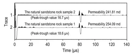
Fig.13 Seismoelectric response in the natural and artificial sandstone samples with similar permeability.

We measured three artificial sandstones with different permeability. From Figure 14, we can see that the amplitude of the seismoelectric signal depends on the permeability of the samples. The amplitude of seismoelectric signal increases with increasingpermeability, which means that the seismoelectric effects are directly related to the permeability and can be used to study the permeability of the reservoir.

Fig.14 Seismoelectric responses in artificial sandstones with different permeability.

Conclusions

In this paper, a seismoelectricity measuring devices were constructed and stable seismoelectric signals were obtained.

It was critical to the seismoelectric measurement to keep the ground potential of the disturbed area of the seismoelectrical conversion consistent with the reference potential of the signal input and maintain a stable reference potential. The antinoise ability of the seismoelectricity measuring system was good as long as the correct critical steps were implemented. The seismoelectrical signal is not easily affected by the noise of the external electrical equipment. The measurement method guarantees the acquisition of the seismoelectric signal and enhances the antinoise performance of the seismoelectric experimental setup.

Control experiments suggest that the obtained signals are attributed to the seismoelectric conversion in the fluid-saturated porous medium. The experimental results confirm that seismoelectric coupling of the seismic wave field and the electromagnetic field is induced in a fluidsaturated porous medium.

The measured seismoelectric signals in saturated sandstone are the seismoelectric interface response of the second-kind seismoelectric effects. The analysis of the attenuation of the seismoelectric signals suggests that the amplitudes of the seismoelectric signals decay exponentially with increasing distance between the electrode and the interface. With increasing distance between the source and the interface, the amplitude of the seismoelectric signals decreases linearly. The energy loss of the seismoelectric signal owing to the increasing distance between the electrode and the sandstone interface is higher than the attenuation of the signal energy owing to the increasing distance between the acoustic source and interface.

The experimental method for measuring the seismoelectrical signal is easy to operate and of good repeatability; furthermore, the recorded signals are clear. The seismoelectric measurement system can obtain stable seismoelectric signals of a few microvolts. The seismoelectric effects induced in artificial sandstone can be used to simulate the seismoelectric effects induced in natural sandstone. The amplitude of the seismoelectric signals increases with increasing permeability. Clearly, the proposed method can be used in modeling seismoelectricity and the petrophysical parameters of reservoirs.

Acknowledgements

We thank Wang Jun for his help with the experiments and Dr. Hu Hengshan for valuable suggestions. This study was supported by the National Science and Technology Major Project (No. 2016ZX05018-005) and New Methods and New Technology Research of Geophysical Prospecting (No. 2014A-3612).

Block, G. I., and Harris, J. G., 2006, Conductivity dependence of seismoelectric wave phenomena in fluidsaturated sediments: Journal of Geophysical Research, 111(B1), 279–288.

Chen, B., and Mu, Y., 2005, Experimental studies of seismoelectric effects in fluid-saturated porous media: Journal of Geophysics and Engineering, 2(3), 222–230.

Deckman, H., Herbolzheimer, E., and Kushnick, A., 2005, Determination of electrokinetic coupling coefficients: 75th Annual International Meeting, SEG, Expanded Abstracts, 561–564.

Dukhin, A. S., Goetz, P. J., and Thommes, M., 2010, Seismoelectric effect: a non-isochoric streaming current. 1. experiment: Journal of Colloid and Interface Science, 345(2), 547–553.

Dukhin, A. S., and Shilov, V. N., 2010, The seismoelectric effect: a nonisochoric streaming current 2. theory and its experimental verification: J. Colloid Interface Sci., 346(1), 248–253.

Gao, Y., and Hu, H. S., 2010, Seismoelectromagnetic waves radiated by a double couple source in a saturated porous medium: Geophys. J. Int., 181, 873–896.

Garambois, S., and Dietrich, M., 2001, Seismoelectric wave conversions in porous media: field measurements and transfer function analysis: Geophysics, 66(5), 1417–1430.

Glover, P. W. J., Ruel, J., Tardif, E., and Walker, E., 2012a, Frequency-dependent streaming potential of porous media—part 1: experimental approaches and apparatus design: International Journal of Geophysics, 2012(1), 1–15.

Glover, P. W. J., Walker, E., Ruel, J., and Tardifet, E.,2012b, Frequency-dependent streaming potential of porous media—part 2: experimental measurement of unconsolidated materials: International Journal of Geophysics, 2012(2), 1–17.

Gershenzon, N. I., Bambakidis, G., and Ternovskiy, I., 2014, Coseismic electromagnetic field due to the electrokinetic effect: Geophysics, 79(5), 217–E229.

Haartsen, M, W., and Pride, S. R., 1996, Electroseismic wave properties: Journal of the Acoustical Society of America, 100(3), 1301–1305.

Haartsen, M. W., and Pride, S. R., 1997, Electroseismic waves from point sources in layered media: Journal of Geophysical Research, 102(B11), 24745–24784.

Haines, S. S., Pride, S. R., Klemperer, S. L. et al., 2007, Seismoelectric imaging of shallow targets: Geophysics, 72(2), G9–G20.

Hu, H. S., and Gao, Y. X., 2011, Electromagnetic field generated by a finite fault due to electrokinetic effect: Journal of Geophysical Research-Solid Earth. 116, B08302.

Lide, D. R., 2010, CRC handbook of chemistry and physics: 90th ed. (Internet), CRC Press/Taylor and Francis.

Pride, S., 1994, Governing equations for the coupled electromagnetics and acoustics of porous media: Physical Review B, 50(21), 15678-5696.

Pengra, D. B., Li, S. X., and Wong, P. Z., 1999, Determination of rock properties by low-frequency AC electrokinetics: Journal of Geophysical Research, 104(B12), 29485.

Revil, A., Jardani, A., Sava, P., and Haas, A., 2015, Theseismoelectricmethod: theory and application: John Wiley & Sons, Ltd, UK, 73–97.

Shaw, D. J., 1992, The solid-liquid interface, introduction to colloid and surface chemistry (4th Edition): Butterworth-Heinemann, 151-173.

Schakel, M. D., Smeulders, D. M. J., Slob, E. C., and Heller, H. K. J., 2011a, Seismoelectric interface response: experimental results and forward model: Geophysics, 76(4), N29–N36.

Schakel, M. D., Smeulders, D. M. J., Slob, E. C., and Heller, H. K. J., 2011b, Laboratory measurements and theoretical modeling of seismoelectric interface response and coseismic wave fields: Journal of Applied Physics, 109(7), 074903.

Schakel, M. D., Smeulders, D. M. J., Slob, E. C., and Heller, H. K. J., 2011c, Seismoelectric fluid/porousmedium interface response model and measurements: Transport in Porous Media, 93(2), 271–282.

Smeulders, D. M. J., Grobbe, N., Heller, H. K. J., and Schakel, M. D., 2014, Seismoelectric conversion for the detection of porous medium interfaces between wetting and nonwetting fluids: Vadose Zone Journal, 13(5), 1539–1663.

Surkov, V. V., Uyeda, S., Tanaka, H., et al., 2002, Fractal properties of medium and seismoelectric phenomena: Journal of Geodynamics, 33(4–5), 477–487.

Thompson, A. H., and Gist, G. A., 1993, Geophysical applications of electrokinetic conversion: The Leading Edge, 12(12), 1169–1173.

Wang, J., Hu, H. S., and Guan, W., 2015a, Experimental measurements of seismoelectric signals in borehole models: Geophys. J. Int., 203, 1937–1945.

Wang, J., Li, H., Hu, H. S. et al., 2015b, Electrokinetic experimental study in borehole model I: the evaluation of rock permeability: Chinese J. Geophys. (in Chinese), 58(10), 3855–3863.

Zhu, Z., Cheng, C. H., and Toksöz, M. N., 1994, Electrokinetic conversion in a fluid-saturated porous rock sample: 64th Annual International Meeting, SEG, Expanded Abstracts, 1057–1060.

Zhu, Z., Haartsen, M. W., and Toksöz, M. N., 1999, Experimental studies of electrokinetic conversions in fluid-saturated borehole models: Geophysics, 64(5), 1349–1356.

Zhu, Z., and Toksöz, M. N., 2003, Crosshole seismoelectric measurements in borehole models with fractures: Geophysics, 68(5), 1519–1524.

Zhu, Z., and Toksöz, M. N., 2005, Seismoelectric and seismomagnetic measurements in fractured borehole models: Geophysics, 70(4), F45–F51.

Zhu, Z., and Toksöz, M. N., 2012, Formation velocity measurements using multipole seismoelectric LWD: Experimental studies: 82th Annual International Meeting, SEG, Expanded Abstracts, 1–6.

Zhu, Z., Toksöz, M. N., and Zhan, X., 2015, Seismoelectric measurements in a porous quartz-sand sample with anisotropic permeability: Geophysical Prospecting, 64(3), 700–713.

Peng Rong Ph.D. candidate in the College of Geophysics and Information Engineering, China University of Petroleum (Beijing). Her main research interests are the seismoelectric effects in fluid-filled porous medium.

Email: hnpengrong@163.com

Manuscript received by the Editor April 25, 2016; revised manuscript received August 20, 2016.

*This work was supported by the National Science and Technology Major Project (No. 2016ZX05018-005) and the New Methods, New Technology Research of Geophysical Prospecting (No. 2014A-3612).

1. State Key Laboratory of Petroleum Resource and Prospecting, Beijing 102249, China.

2. CNPC Key Laboratory of Geophysical Exploration, Beijing 100083, China.

3. Institute of Geophysics and Information Engineering, China University of Petroleum (Beijing), Beijing 102249, China.

♦Corresponding author: Ding Pin-Bo (Email: dingpinbo@163.com)

© 2016 The Editorial Department of APPLIED GEOPHYSICS. All rights reserved.