Three-dimensional forward modeling and inversion of borehole-to-surface electrical imaging with different power sources*

Bai Ze, Tan Mao-Jin♦,2, and Zhang Fu-Lai

Three-dimensional forward modeling and inversion of borehole-to-surface electrical imaging with different power sources*

Bai Ze1, Tan Mao-Jin♦1,2, and Zhang Fu-Lai3

Borehole-to-surface electrical imaging (BSEI) uses a line source and a point source to generate a stable electric field in the ground. In order to study the surface potential of anomalies, three-dimensional forward modeling of point and line sources was conducted by using the finite-difference method and the incomplete Cholesky conjugate gradient (ICCG) method. Then, the damping least square method was used in the 3D inversion of the formation resistivity data. Several geological models were considered in the forward modeling and inversion. The forward modeling results suggest that the potentials generated by the two sources have different surface signatures. The inversion data suggest that the lowresistivity anomaly is outlined better than the high-resistivity anomaly. Moreover, when the point source is under the anomaly, the resistivity anomaly boundaries are better outlined than when using a line source.

Borehole-to-surface electrical imaging, different types of exciting sources, potential characteristic, forward modeling, resistivity inversion

Introduction

Borehole-to-surface electrical imaging (BSEI) establishes a stable electric field by applying current through the borehole casing or via a power source inside the borehole (Dey and Morrison, 1979; Scriba, 1981; Beasley and Ward, 1986). When there is an underground anomaly, the electric field changes. Owing to the power supply that is directly in contact with the target layer, BSEI has higher vertical resolution and penetrates deeper than conventional electrical prospecting methods (Tsili et al., 1991; Bevc and Morrison, 1991). In recent years, BSEI has been widely used in monitoring the effects of water injection and fracturing in oil fields, and looking for ore and groundwater (Nimmer and Osiensky, 2002; Surendra, 2004; Tan et al., 2004; David et al., 2008; Perri et al., 2012; Lorenzo et al., 2013; Zhang et al., 2014; Thomas et al., 2015).

Numerical modeling of BSEI is used in datainterpretation and inversion. Generally, the finitedifference method (FDM) and finite-element method (FEM) are used for that purpose. Mizunaga and Ushijima (1991) performed 3D forward modeling of a vertical line source by using the FDM and analyzed the surface potential. Spitzer (1995) introduced the conjugate gradient method into a 3D finite-difference algorithm and used a compact storage scheme that converged fast and required less computer storage. However, the burial depth, size, and electrical differences with the surrounding medium of the anomalous body strongly affect the surface potential, Chen (2009) enhanced the response of the anomaly by carrying out the directional derivation of the potential. Su et al. (2012) combined borehole–surface potential and crosswell potential data obtained by numerical simulation to successfully determine the spatial distribution of the remaining oil. Gu et al. (2015) used the Archie equation to establish the relation between oil–water two-phase flow and electric field, and obtained the one-dimensional well–ground potential and the relation between the potential and residual oil saturation by using the FDM. Compared with the FDM, the FEM requires higher computer storage and computational time (Li and Spitzer, 2002). Based on the FEM, Wu (2003) developed an algorithm by using the row-indexed sparse storage mode to store the coefficient matrix and the shifted incomplete Cholesky conjugate gradient (SICCG) iterative method to solve the large linear equations, greatly improving the computational speed and reducing the storage space. However, the actual formation model is anisotropic or heterogeneous, Li and Spitzer (2005) presented a 3D finite-element algorithm for nearly arbitrary structures, including general anisotropy. Liu et al. (2011) performed 3D numerical forward modeling of the continuous changes in the electric field and analyzed the investigation depth of the BSEI using a line source. In numerical simulations of BSEI using a point source, the FDM and FEM were also used (Pridmore et al., 1981; Zhou et al., 1986; Wu et al., 1998; Chen, 2012; Dai et al., 2013). In addition, the distribution of the electric field and surface potential using a line source and point source in experiments (Wang et al., 2005; Du et al., 2013) formed the basis for future numerical simulations.

For resistivity inversion, Loke and Barker (1995) proposed a least squares deconvolution method that produces distortion-free inversion results; the distortion is due to the electrode array geometry. It is important and necessary to consider the storage needs for the Jacobian matrix and the inversion calculation efficiency. Using the conjugate gradient (CG) relaxation to solve the equations avoids calculating the Jacobian matrix, which reduces the demand for computer memory and improves the speed (Wu and Xu, 2000; Lian, 2007). Tan et al. (2004) used least squares to invert borehole-to-surface resistivity data from the eighth section of the Gudong Oilfield and studied the distribution of residual oil. Ho (2009) performed 3D resistivity inversion using borehole-tosurface electrical data from the Takigami area in Japan and neural networks. Tsourlos et al. (2011) introduced an extra weighting factor to the smoothness-constrained inversion method and improved the precision. Tsourlos et al. (2014) used the 2.5D finite-element method to solve Poisson’s equation, and proposed a fast and efficient inversion for two-dimensional resistivity tomography. Zhou (2015) inverted borehole-to-surface resistivity from a point source by using the reweighted regularized conjugate gradient method, and improved the stability and convergence rate.

In summary, the abovementioned studies focused on the forward modeling and resistivity inversion using BSEI and single-point or single-line sources, but there is no comparison of the different excitation sources. Forward modeling and resistivity inversion using BSEI and different excitation sources not only provides the theoretical framework for data interpretation but also determines which power source is better to identify anomalies. In this study, the finite-difference method was used in 3D modeling of BSEI and different excitation sources, and the damping least square method in resistivity inversion. For different geological models, the surface potential of the anomalies was analyzed and the inverted resistivity of different excitation sources was compared.

Forward modeling of the anomaly potential

Separation of the anomaly potential

The 3D numerical simulation of BSEI satisfies the basic differential equations of the direct current method, namely, Poisson’s equation (Dey and Morrison, 1979)

where the right side of the equation is the current source, σ represents the electrical conductivity of the formation, u is the potential, I is the current, δ is the Dirac function, (x0, y0, z0) is the location of the source, and (x, y, z) is the location of observed point.

In numerical simulations, to eliminate the singular values owing to the source, the total potential is separated into normal and anomalous (LeMasne and Poirmeur, 1988)

where utrepresents the total potential, upis the normal potential, which is singular and caused by the current source, and usrepresents the anomalous potential owing to the underground anomalous body.

The average conductivity of the formation is σ0and upalso conforms to equation (1)

By substituting equations (2) and (3) into equation (1), the differential equation of the anomalous potential is obtained

In homogeneous media, the normal potential owing to a point source and an arbitrary line source upis derived from “mirror theory.” The theoretical potential of an arbitrary point M in space produced by the point source is (Chen, 2009)

where r and r' is the distance of point source A and its virtual point source A' to point M in space, respectively, and σ0is the conductivity of the homogeneous halfspace.

Based on equation (5), the normal potential of arbitrary point M on the ground produced by a point source is

where r is the distance of the point source to the observation point on the ground.

The line source is considered the linear superposition of countless point sources (Mizunaga and Ushijima, 1991), and the normal potential of arbitrary point M in space produced by the arbitrary line source is

where

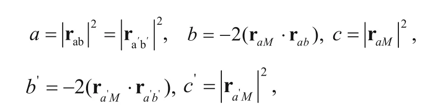
when point M is on the surface,

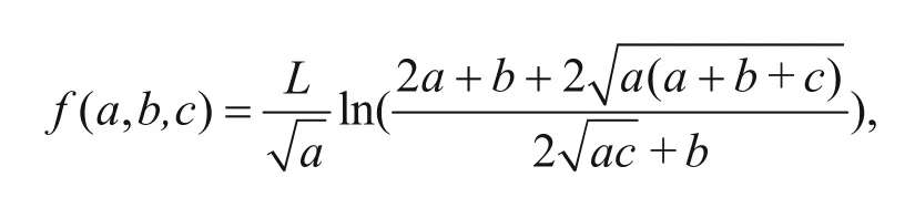
and

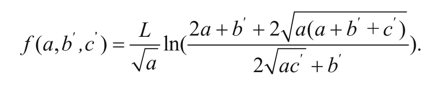
The specific corresponding relation of the vectors is shown in the Figure 1.

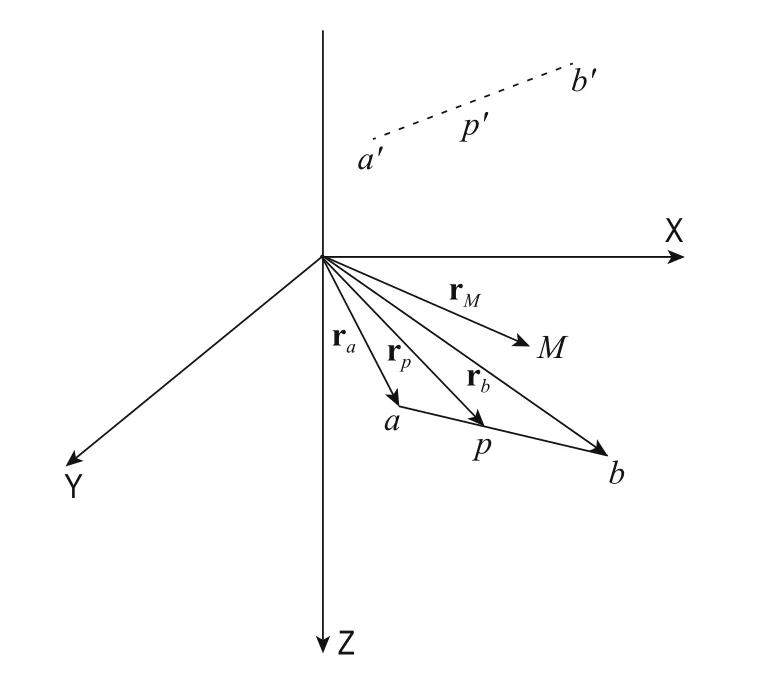
Fig.1 Normal potential diagram for arbitrary underground line sources.

Anomaly potential by the finite-difference method

The finite-difference method was used to calculate the anomaly potential. The target space is divided into rectangular M × N × L grids. Each vertex of the grid is called a node, and we use the potential at the nodes to represent the continuous potential function in the target space. The nodes in the X-direction are i = 1, 2, …, M, the nodes in the Y-direction are denoted as j = 1, 2, …, N, and the nodes in the Z-direction are k = 1, 2, …, L. Based on the finite-difference method, equation (4) is written as follows (Zhang, 2009):

where Ctop, Cbottom, Cright, Cleft, Cfront, Cback, and Cmiddleare the coefficients of the relation of node (i, j, k) with the top node, bottom node, right node, left node, front node, and back node, respectively. All nodes have the form of equation (8). Finally, M × N × L equations are derived for numerical analysis and are simplified in matrix form

where the coefficient matrix C is a large sparse symmetric positive-definite matrix, which is related to the geometric properties of the grids and the distribution of conductivity,is the anomaly potential, andis the normal potential vector that has zero values at the nonpowered nodes.

The incomplete Cholesky conjugate gradient (ICCG) method is subsequently used to solve the linear equation (9), and obtain the anomalous potential at each node. The normal potential is calculated analytically and the total potential is obtained by using equation (2).

The equation for the apparent resistivity is

where utis the total potential, and k is the coefficient of the apparatus and different apparatuses have different coefficients (Dey and Morrison, 1979). In this study, pole–pole observations are used.

The first and second boundary conditions are considered in the numerical simulation. At the surface, the air acts as insulator and the current density j is zero. Becauseand, the second boundary condition on the surface isand the other boundary is u = 0.

Method verification

The resistivity of a homogenous half-space is set at 100 Ω·m and divided into 10 m × 10 m × 10 m grids. The point source is at 100 m depth, the top depth of the vertical line source is 5 m, and the bottom depth is 100 m. The power-supplied current is 2 A, and 12 points were set on the ground on the right side of the current source and in the positive direction of the X-axis. The numerically and analytically calculated subsurface potentials are compared in Figure 2. Figures 2a and 2b show that the numerical and analytical solutions for the point and line sources fit the data well.

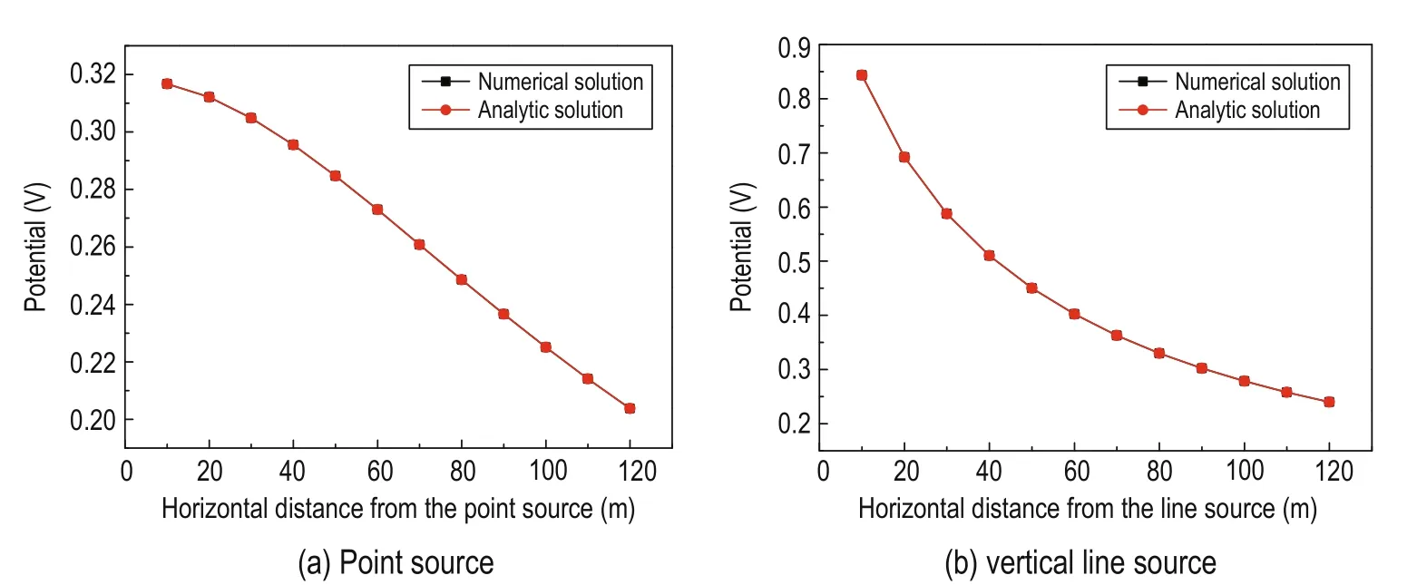
Fig.2 Numerical and analytical fitting solutions to the data.

Resistivity inversion method

In the 3D resistivity inversion, we used the forward modeling approach. The resistivity inversion problem can be expressed as (Wu and Xu, 2000)

whereoc

Δ = -d d d represents the residuals, Δm is the modification vector of m0, and G is the Jacobianmatrix. In the inversion, the range of the inversion data and model parameters is large, which results in an extremely unstable Jacobian matrix G. To solve this problem, we take the logarithm of the inverted data and the model parameters and writeandTo ensure the stability of the inversion, we use the

Δ Δm m minimum as constraint and the objective function of the inversion is

where λ is the damping factor. We minimize the objective function φ

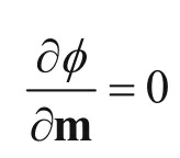
to obtain

It is important to select an appropriate dampingfactor λ; thus, Wu and Xu (2000) analyzed the inversion stability and convergence by using different λ factors. When λ is 0.05, the inversion converged quickly and stably. Thus, we chose to use λ = 0.05. Δm was obtained by solving equation (13). To modify the initial guess model m0, we used the modified model in the iterations until the convergence condition was satisfied. The inversion steps are shown in Figure 3.

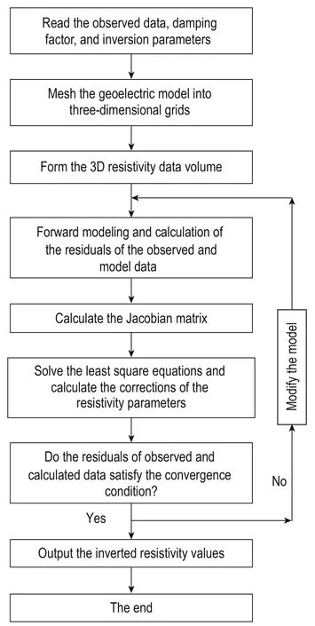
Fig.3 Inversion flow chart.

Numerical example

Forward modeling

In order to compare and study the surface response of an anomaly using different excitation sources, we designed different numerical models to simulate and analyze the response characteristics. We used the nonuniform grid mesh method for a 10 km×10 km × 5 km area and an area of observation of 2 km ×2 km. The mesh grids were 60 × 60 × 46 and most grids were 50 m × 50 m × 50 m. The current was 10 A. The simulation results are discussed below.

Point source

Point sources are widely used in barefoot wells. We placed the anomaly at different depths to analyze the ground response. The resistivity of the surrounding rock was set at 100 Ω·m, whereas the resistivity of the 1000 m × 200 m × 100 m anomaly was set at 10 Ω·m. The point source was located at 1000 m, and the center of the anomaly was at 500 m, 1000 m, and 1500 m depth.

Figure 4a shows the projection of the model on the XOZ plane. I, II, and III mark the location of the anomaly at the different depths, and the red dot marks the location of the point source. Figures 4b, 4c, and 4d show the contour maps of the anomaly potential on the ground. The red is for high potential, the blue for low potential, and the white dotted rectangular represents the projection of the anomaly on the ground.

Figure 4b shows that when the point source is below the anomaly, the surface potential is positive, and the high potential is at the center and extends along the anomaly. The left and right boundaries of the anomaly are characterized by two positive maxima and outline the anomaly. In Figure 4c, we can see that when the point source is excited in a low-resistivity body, the central area of the anomaly on the surface is characterized by negative minima and is surrounded by high potential. The long axis of the anomaly corresponds to the short axis of the negative potential, and the left and rightboundaries of the anomaly are at the transitional region from negative to positive potential. Figure 4d shows the point source above the anomaly, where the potential values are all negative and the relation between the potential and the anomaly is unclear and the anomaly is unidentifiable.

Based on the numerical simulation of the point source, the position of the source relative to the anomaly and the surface potential are related. Hence, the anomaly can be reflected by the potential on the surface when the excited source is in the anomaly or below it.

Fig.4 Surface potential of the model anomaly at different depths.

Vertical line source

In oil fields, the effects of water injection and fracturing are monitored by using BSEI. Power is often supplied directly through the casing, and the casing is the line source. To examine this case, the resistivity of the surrounding rock and anomaly were set the same as in the point-source model. The length of the line source was set at 1000 m, the dimensions of the anomaly were 1000 m × 200 m × 100 m, the distance from the left boundary of the anomaly to the line source was 200 m, and the distance from the right boundary of the anomaly to the line source was 800 m. The anomaly was set the depth of 500 m, 950 m, and 1200 m.

Figure 5a shows the projection on the XOZ plane. I, II, and III mark the position of the anomaly at different depths. The red solid line represents the line source. Figures 5b, 5c, and 5d show contour maps of the potential of the anomaly on the ground.

In Figure 5, we can see that the shape of the anomaly potential gradually fades and the potential on the ground decreases with increasing burial depth of the anomaly. When the anomaly is well below the line source, the anomaly potential on the surface is negative. The boundaries of the anomaly are clearly identified whenthe line source goes through the anomaly, and the left and right boundaries of the anomaly close at the negative and positive extremes. The direction of the maximum potential corresponds to the extended direction of the anomaly; hence, BSEI with a vertical line source can be used to identify the predominant direction of water flooding and fracturing.

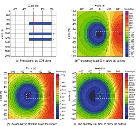
Fig.5 Surface potential of the model anomaly at different depths.

Slant line source

In practice, a slant line source is occasionally used. Thus, we used line sources with angle of inclination of 0°, 30°, 45°, and 60°. The burial depth of the anomaly was set at 700 m, whereas the length of the line source and the other parameters were the same as in the vertical line source.

Figures 6a and 6b show the projection of the model on the XOZ and YOZ plane, respectively. A simple situation is considered where the line source is only inclined along the negative direction of the Y-axis in the YOZ plane. Figures 6c, 6d, 6e, and 6f show contour maps of the anomaly potential on the surface. The red dotted line denotes the projection of the line source on the ground.

Figure 6 shows that as the inclination of the line source increases along the negative direction of the Y-axis, the maximum of the potential gradually moves along the positive direction of the Y-axis. Therefore, if the line source is inclined, the effect of the angle of inclination on the potential must be considered when evaluating the position and direction of the anomaly.

Inversion

We built different geological models of point and vertical line sources, performed resistivity inversion at different depths, and compared the inversion results. The calculation of the Jacobian matrix is computationally costly. To reduce the computer memory requirements, weconsidered an area of 2 km × 2 km × 1.5 km and 20 × 20 × 16 mesh grids. The 0.8 km × 0.8 km area of observation was located at the center. Finally, the same mesh as in the forward modeling was used in the inversion.

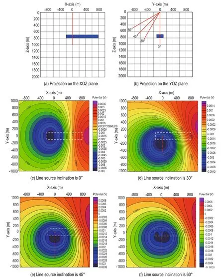
Fig.6 Surface potential of the model anomaly for a variably inclined line source.

Model I

The low resistivity of the anomaly is set at 10 Ω·m and the high at 1000 Ω·m, whereas the resistivity of the surrounding rock is 100 Ω·m. The anomaly dimensions are 200 m × 200 m × 100 m and is buried at 300 m depth, whereas the point source is below the anomaly at 500 m depth. The vertical line source is 500 m long and the current is 10 A.

Figure 7a shows the projection of the model on the ground, and Figures 7b, 7c, and 7d show the contours ofthe resistivity inversion results for point source at 300 m, 500 m, and 700 m depth, respectively. Similarly, Figures 7e, 7f, and 7g show the contours of the resistivity inversion result for the vertical line source.

In Figure 7, we can see that the resistivity results show the position of the low-and high-resistivity body; however, the low-resistivity body is more clearly identified. With increasing depth, the boundaries of the anomaly gradually diverge but still outline the anomaly. In addition, the point source yields better results than the line source.

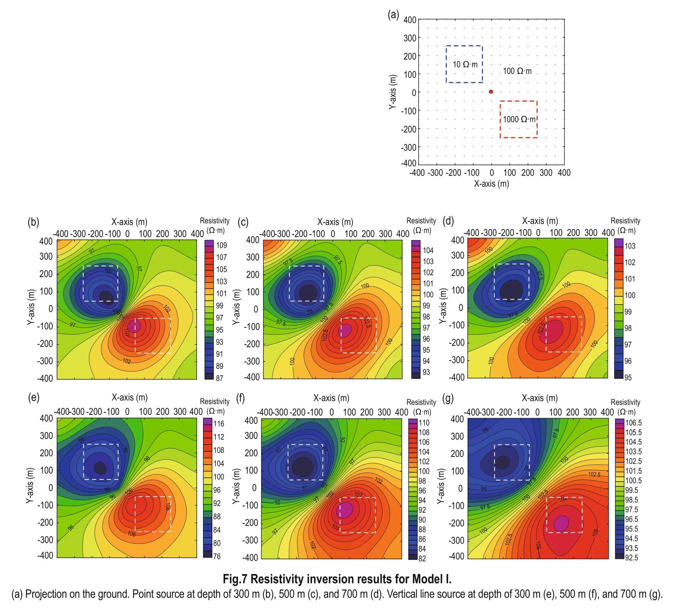
Fig.7 Resistivity inversion results for Model I.

Model II

We built model II considering two low-resistivity bodies. The other parameters are the same as model I.

Figure 8a shows the projection of the model on the ground. Figures 8b, 8c, and 8d show the resistivity contour maps for a point source at 300 m, 500 m, and 700 m depth, respectively, where as Figures 8e, 8f, and 8g show the resistivity contour maps for a vertical line source at the same depths.

In Figure 8, we see that the inverted resistivity for a point source outlines the anomaly, whereas the linesource inversed resistivity has errors. Nevertheless, both outline the anomaly despite the model shortcomings.

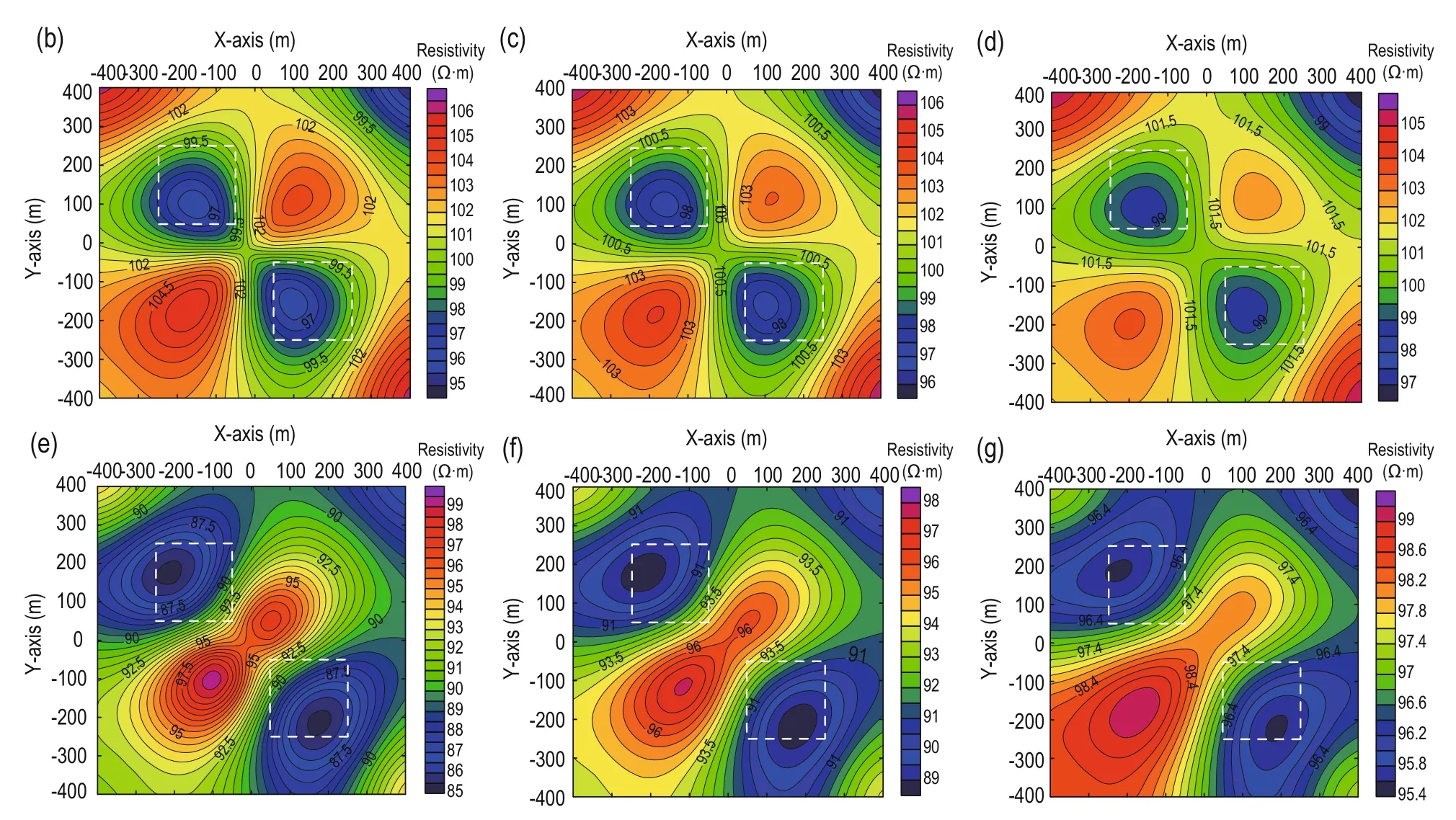
Fig.8 Inverted resistivity at different depths for the point and line sources in Model II.

Conclusions

Borehole-to-surface electrical imaging is a direct current prospecting method that is simple, practical, fast, and efficient. It has high sensitivity to the electrical properties of the geological formations and can be used in dynamic monitoring. In this study, forward modeling and inversion of BSEI data using point and line sources were performed.

The finite-difference method can be used in 3D numerical simulations of borehole-to-surface electrical imaging for different types of power sources. The numerical simulation results directly correspond to the anomaly and suggest that BSEI can be used to detect underground anomalies.

When the excitation source is in the borehole, the surface signature of the anomaly potential depends on the location of the source. By combining the location of the source and the characteristics of the anomaly potential on the surface, we determine the position of the anomaly semi-quantitatively. In addition, the position and boundaries of the anomaly are better outlined when a point source in or below the anomaly.

The direction of the maximum anomaly potential on the surface corresponds to the long dimension of the anomaly when the power is supplied through the vertical borehole casing. When the power supplied to the casing is slant, the maximum anomaly potential on the surface moves opposite to the casing inclination direction.

The inversion results show that the resistivity outlines the position of the anomaly. However, the low-resistivity body is better outlined than the high-resistivity body. Furthermore, a point source underneath the anomaly produces more precise results than a line source in the same formation.

Acknowledgements

The authors express their sincere thanks to Drs Zhang Yuanzong, Gao Jie, and Wang Xiaochang for constructive comments and suggestions that greatly improved the manuscript.

Beasley, C. W., and Ward, S. H., 1986, Tree-dimensional mise-a-la-masse modeling applied to mapping fracture zones: Geophysics, 51(1), 98-113.

Bevc, D., and Morrison, H. F., 1991, Borehole-to-surface electrical resistivity monitoring of salt water injection experiment: Geophysics, 56(6), 769-777.

Chen, D. P., 2009, 3D FEM forward modeling research of borehole-to-surface DC method drived by the arbitrary linear current source: Msc Thesis, Central South University, Hunan.

Chen, Y. X., 2012, Three-dimensional FEM numerical simulation of borehole-ground potential with gradient current source: Msc Thesis, Central South University, Hunan.

Dai, Q. W., Hou, Z. C., and Wang, H. H., 2013, Analysis of anomaly of Borehole-to-surface electrical method by 2.5D finite element numerical simulation: Geophysical Computing Technology, 35(4), 458-462.

David, P., Carlos, T. V., and Zhang, Z. Y., 2008, Sensitivity study of borehole-to-surface and crosswell electromagnetic measurements acquired with energized steel casing to water displacement in hydrocarbonbearing layers: Geophysics, 73(6), 261-268.

Dey, A., and Morrison, H. F., 1979, Resistivity modeling for arbitrarily shaped two-dimensional structures: Geophysical Prospecting, 27(1), 106-136.

Du, L. Z., Jiang, X. M., Qu, J. W., et al., 2013, Experimental study on abnormal electric field distribution of surfaceborehole electrical method: Global Geology, 3(32), 558-589.

Gu, J. W., Li, F. J., Liu, Y., et al., 2015, Establishing and solving of a one-dimensional well-ground potential model: Journal of China University of Petroleum, 39(6), 100-102.

Ho, T. L., 2009, 3-D inversion of borehole-to-surface electrical data using a back-propagation neural network: Journal of Applied Geophysics, 68(4), 489-499.

LeMasne, D., and Poirmeur, C., 1988, Three-dimensional model results for an electrical hole-to-surface method: Application to the interpretation of a filed survey: Geophysics, 53(1), 85-103.

Li, Y. G., and Spitzer, K., 2002, Tree-dimensional DC resistivity forward modeling using finite elements in comparison with finite-difference solutions: Geophysics Journal International, 151(3), 924-934.

Li, Y. G., and Spitzer, K., 2005, Finite element resistivity modeling for three-dimensional structures with arbitrary anisotropy: Physics of the Earth and Planetary Interiors, 150(1-3), 15-27.

Lian, J., 2007, Research on forward modeling and inversion of vertical line source borehole-ground DC method: M sc Thesis, China University of Geosciences (Beijing), Beijing.

Liu, H. F., Chen, D. P., Dai, Q. W., et al., 2011, 3D FEM modeling of borehole-surface potential with line current source in semi-underground space of continuous variation of conductivity: Journal of Guilin University of Technology, 31(1), 29-38.

Loke, M. H., and Barker, R. D., 1995, Least-squares deconvolution of apparent resistivity pseudosections: Geophysics, 60(6), 1682-1690.

Lorenzo, D. C., Maria, T. P., Maria, C. C., et al., 2013, Characterization of dismissed landfill via electrical resistivity tomography and mise-a-la-masse method: Journal of Applied Geophysics, 98, 1-10.

Mizunaga, H., and Ushijima, K., 1991, Three-Dimensional numerical modeling for the mise-a-la-masse method: Geophysical Exploration (Butsurib-Tansa), 44(4), 215-226.

Nimmer, R. E., and Osiensky, J. L., 2002, Using mise-a-lamasse to delineate the migration of conductive tracer in partially saturated basalt: Environmental Geosciences, 9(2), 8-87.

Perri, M. T., Cassiani, G., Gervasio, I., et al., 2012, A saline tracer test monitored via both surface and cross-borehole electrical resistivity tomography: comparison of timelapse results: Journal of Applied Geophysics, 79, 6-16.

Pridmore, D. F., Hohmann, G. W., Ward, S. H., et al., 1981, An investigation of finite-element modeling for electrical and electromagnetic data in three dimensions: Geophysics, 46(7), 1009-1024.

Scriba, H., 1981, Computation of the electrical potential in three dimension structures: Geophysical Prospecting, 29(5), 790-802.

Spitzer, K., 1995, A 3-D finite-difference algorithm for DC resistivity modeling using conjugate gradient methods: Geophysical Journal International, 123(3), 903-914.

Su, B. Y., Fujimitsu, Y., Xu, J. L., et al., 2012, A model study of residual oil distribution jointly using crosswell and borehole-surface electric potential methods: Applied Geophysics, 9(1), 19-26.

Surendra, R. P., 2004, Tracing groundwater flow by misea-la-masse measurement of injected saltwater: Journal of Environmental and Engineering Geophysics, 9(3), 155-165.

Tan, H. Q., Shen, J. S., Zhou, C., et al., 2004, Borehole-tosurface electrical imaging technique and its application to residual oil distribution analysis of the eighth section in Gudong Oilfield: Journal of the University of Petroleum, China, 28(2), 32-37.

Thomas, H., Andreas, K., and Frederic, N., 2015, Covariance-constrained difference inversion of timelapse electrical resistivity tomography data: Geophysics, 81(5), 311-322.

Tsili, W., Stodt, J. A., Stierman, D. J., et al., 1991, Mapping hydraulic fracture using a borehole-to-surface electrical resistivity method: Geoexploration, 28(3-4), 349-369.

Tsourlos, P., Ogilvy, R., Papazachos, C., et al., 2011, Measurement and inversion schemes for single borehole–to-surface electrical resistivity tomography surveys: Geophysics and Engineering, 8(4), 487-497.

Tsourlos, P., Papadopoulos, N., Papazachos, C., et al., 2014, Efficient 2D inversion of long ERT section: Journal of Applied Geophysics, 105, 213-224.

Wang, Z. G., He, Z. X., Wei, W. B., et al., 2005, 3-D physical model experiments of well-to-ground electrical survey: Oil Geophysical Prospecting, 40(5), 595-597.

Wu, X. P., 2003, A 3-D finite-element algorithm for DC resistivity modeling using the shifted incomplete Cholesky conjugate gradient method: Geophysical Journal International, 154(3), 947-956.

Wu, X. P., and Xu, G. M., 2000, Study on 3-D resistivity inversion using conjugate gradient method: Chinese Journal of Geophysics, 43(3), 421-426.

Wu, X. P., Xu, G. M., and Li, S. C., 1998, The calculation of Three-dimensional geoelectric field of point source by incomplete Cholesky conjugate gradient method: Acta Geophysica Sinica, 41(6), 848-855.

Zhang, Y. Y., Liu, D. J., Ai, Q. H., et al., 2014, 3D modeling and inversion of the electrical resistivity tomography using steel cased boreholes as long electrodes: Journal of Applied Geophysics, 109, 292-300.

Zhang, Y., 2009, The forward modeling of Threedimensional borehole-to-surface logging technology: MSc thesis, Ocean University of China, Qingdao.

Zhou, X. R., Zhong, B. S., Jiang, Y. L., et al., 1986: Numerical simulation technology of electrical prospecting, Sichuan Science and Technology Press, Chengdu, 163-239.

Zhou, Y. Q., 2015, 2.5-D modeling and inversion of the surface to hole resistivity imaging research and application: Msc Thesis, East China Institute of Technology, Jiangxi.

Bai Ze, a PhD Candidate of the School of Geophysics and Information Technology, China University of Geosciences (Beijing). His research interests are in electrical prospecting and well logging.

Email: 2010140038@cugb.edu.cn.

Manuscript received by the Editor January 28, 2016; revised manuscript received September 3, 2016.

*This work was sponsored by the National Major Project (No. 2016ZX05014-001), the National Natural Science Foundation of China (No. 41172130 and U1403191), and the Fundamental Research Funds for the Central Universities (No. 2-9-2015-209).

1. School of Geophysics and Information Technology of China University of Geosciences, Beijing 100083, China.

2. Key laboratory of Geo-detection (China University of Geosciences), Ministry of Education, Beijing 100083, China.

3. Beijing Horizontal Hualong Technology Ltd., Beijing 100049, China.

♦Corresponding author: Tan Mao-Jin (Email: tanmj@cugb.edu.cn)

© 2016 The Editorial Department of APPLIED GEOPHYSICS. All rights reserved.