Evaluation of the Tropical Variability from the Beijing Climate Center's Real-Time Operational Global Ocean Data Assimilation System

Wei ZHOU,Mengyan CHEN,Wei ZHUANG,Fanghua XU,Fei ZHENG,Tongwen WU,and Xin WANG

1Laboratory for Climate Studies,National Climate Center,China Meteorological Administration,Beijing 100081

2State Key Laboratory of Tropical Oceanography,South China Sea Institute of Oceanology, Chinese Academy of Sciences,Guangzhou 510301

3Ministry of Education Key Laboratory for Earth System Modeling,and Center for Earth System Science,

Tsinghua University,Beijing 100084

4International Center for Climate and Environment Science,Institute of Atmospheric Physics, Chinese Academy of Sciences,Beijing 100029

Evaluation of the Tropical Variability from the Beijing Climate Center's Real-Time Operational Global Ocean Data Assimilation System

Wei ZHOU∗1,Mengyan CHEN2,Wei ZHUANG2,Fanghua XU3,Fei ZHENG4,Tongwen WU1,and Xin WANG2

1Laboratory for Climate Studies,National Climate Center,China Meteorological Administration,Beijing 100081

2State Key Laboratory of Tropical Oceanography,South China Sea Institute of Oceanology, Chinese Academy of Sciences,Guangzhou 510301

3Ministry of Education Key Laboratory for Earth System Modeling,and Center for Earth System Science,

Tsinghua University,Beijing 100084

4International Center for Climate and Environment Science,Institute of Atmospheric Physics, Chinese Academy of Sciences,Beijing 100029

The second-generation Global Ocean Data Assimilation System of the Beijing Climate Center(BCCGODAS2.0)has been run daily in a pre-operational mode.It spans the period 1990 to the present day.The goal of this paper is to introduce the main components and to evaluate BCCGODAS2.0 for the user community.BCCGODAS2.0 consists of an observational data preprocess,ocean data quality control system,a three-dimensional variational(3DVAR)data assimilation,and global ocean circulation model[Modular Ocean Model 4(MOM4)].MOM4 is driven by six-hourly fluxes from the National Centers for Environmental Prediction.Satellite altimetry data,SST,and in-situ temperature and salinity data are assimilated in real time.The monthly results from the BCCGODAS2.0 reanalysis are compared and assessed with observations for 1990-2011. The climatology of the mixed layer depth of BCC GODAS2.0 is generally in agreement with that of World Ocean Atlas 2001. The modeled sea level variations in the tropical Pacific are consistent with observations from satellite altimetry on interannual to decadal time scales.Performances in predicting variations in the SST using BCC GODAS2.0 are evaluated.The standard deviation of the SST in BCC GODAS2.0 agrees well with observations in the tropical Pacific.BCCGODAS2.0 is able to capture the main features of El Nin˜o Modoki I and Modoki II,which have different impacts on rainfall in southern China.In addition,the relationships between the Indian Ocean and the two types of El Nin˜o Modoki are also reproduced.

operational oceanography,global ocean,3DVAR,El Nin˜o,interannual variability

1.Introduction

Ocean initialization plays a critical role in short-term climate prediction because most predictive skill comes from the initial conditions of the upper ocean,particularly that associated with large-scale variability,such as ENSO and the Indian Ocean Dipole(IOD)(Alves et al.,2011).A common strategy to obtain the optimal initialization of the ocean is to assimilate the available ocean observations into ocean models forced by atmospheric fluxes(Xue et al.,2011;Zheng and Zhu,2015).Various assimilation methods have been applied for the initialization of operational or quasi-operational coupled forecast systems.For example,a three-dimensionalvariational(3DVAR)analysis with a temporally and spatially varying background error covariance is used in the global ocean data assimilation system(GODAS)of the National Centers for Environmental Prediction(NCEP)(Behringer et al.,1998).In version 3 of the ECMWF(European Centre for Medium-Range Weather Forecasts)ocean analysis system,the incremental 3DVAR method is applied(Balmaseda et al.,2013).A more advanced data assimilation method, the EnKF(Ensemble Kalman Filter),has been employed in TOPAZ4(the latest version of TOPAZ-a coupled ocean-sea ice data assimilation system for the North Atlantic Ocean and Arctic),which can make background error covariance vary with time(Sakov et al.,2012).Noticeably,the data assimilation in these systems is performed separately for ocean and atmosphere models in order to achieve optimal initialization (Zheng et al.,2009;Alves et al.,2011).

©Institute of Atmospheric Physics/Chinese Academy of Sciences,and Science Press and Springer-Verlag Berlin Heidelberg 2016

High-quality in-situ and remote sensing data with fine spatial and temporal resolution are crucial for the development of a global operational ocean data assimilation system (Han et al.,2013;Ratheesh et al.,2014).Satellite observations of the ocean,which provide global coverage and realtime measurements of sea level,SST,sea ice,waves,and winds,have become a primary data source for operational oceanography.The launch of TOPEX/Poseidon(T/P)has provided an accurate description of the large-scale sea level and ocean circulation for the first time since 1992.The altimetry products at higher resolution have been supplied following the launch of ERS-1/2,Janson-1 and ENVISAT(Hunt et al.,2007).SST is an important variable for operational oceanography and for assimilation into global ocean models because SST is strongly related to air-sea interactions and can be used to correct errors in forcing fields(e.g.,wind and surface heat fluxes).Satellite-derived SST products are available in two types,according to the sensors equipped on satellites.Optical/infrared data,including data from the Advanced Very High Resolution Radiometer(AVHRR),are affected by clouds and volcanic aerosols in the atmosphere (Reynolds and Marsico,1993).Microwave data can be obtained through non-precipitating clouds and are very beneficialintermsofgeographicalcoverage(Ratheeshetal.,2014). However,satellite observations are mainly confined to surface information.In-situ observations can complement satellite observations by providing measurements below the ocean surface.This is especially true of the Array for Real-time Geostrophic Oceanography(ARGO)project,which has been established since 2000 and now provides important in-situ observations to validate satellite data and improve the initialization of ocean models.ARGO floats measure the temperature and salinity in the upper 2000 m of the ocean and bring unquestionable advances to ocean forecast models(Huang et al.,2008).The joint use of high resolution satellite observations and high accuracy in-situ observations fulfills the operational requirements for temporal and spatial coverage and near real-time access.

A new generation of short-term climate forecast systems is being developed at the Beijing Climate Center(BCC CSM1.1)(Wu et al.,2013,2014),and the access to initial oceanic conditions depends on the development of a global ocean data assimilation system.The first generation of the global ocean data assimilation system of the Beijing Climate Center(BCC GODAS1.0)has been developed during the period from January 1996 to December 2000,has been operational since 2002(Liu et al.,2005),and plays an important role in climate forecast services.With the development of satellite technology and the data assimilation method,some limitations of BCC GODAS1.0 have gradually emerged,especially with regard to not assimilating satellite observations. The physical processes in the BCC GODAS1.0 ocean model and the ocean component used in BCC CSM1.1 are different.A new method for assimilating altimeter and SST data under one dynamic constraint based on 3DVAR was developed to solve the problem of multivariate assimilation (Wang et al.,2012a,2012b).The new method has been implemented into BCC GODAS2.0,which now has the ability to assimilate real-time observations and to run automatically.The physical processes and grid of the ocean model used in BCC GODAS2.0 are the same as those used in BCC CSM1.1.Therefore,the ocean initialization field generated by BCC GODAS2.0 can be used in BCCCSM1.1 directly. The global ocean reanalysis products of BCCGODAS2.0 are being applied in BCC CSM1.1.

This paper is organized as follows:Section 2 provides an overview of the configurations of the ocean model and the 3DVAR analysis scheme,as well as the ocean observations used in the assimilation.Section 3 discusses the model performance and interannual-to-decadal variability in the tropical Pacific.A summary and conclusions are given in section 4.

2.The operational ocean system

2.1.The ocean model

The ocean model used in BCC GODAS2.0 is version 4 of the Modular Ocean Model(MOM4),developed at the Geophysical Fluid Dynamics Laboratory(Griffies et al.,2003). Its zonal resolution is 1◦,while the resolution in the meridional direction is 1/3◦within 10◦of the equator,smoothly increasing to 1◦in the poleward direction of 30◦.There are 50 z-levels in the vertical direction,with a 10 m resolution from the surface to a depth of 225 m,gradually increasing to approximately 366 m in the abyssal zone.The maximum depth is approximately 5.5 km.The tripolar grid is adopted to avoid a singularity at the North Pole(Griffies et al.,2005). The two north poles of the curvilinear grid are situated over land areas in North America and Eurasia,respectively.The model uses identical physical parameterization schemes as described in Griffies et al.(2005),including the isopycnal tracer mixing and diffusion scheme,the Laplace horizontal friction scheme,and the K-Profile Parameterization vertical mixing scheme.The model is forced with 6-h averaged 10-m wind and 2-m air temperature data from the NCEP/NCAR (National Center for Atmospheric Research)Reanalysis I dataset(http://www.esrl.noaa.gov/psd/).The mean climatological river runoff is specified at the coastlines of the model. Surface temperature and salinity are relaxed to monthly Levitus climatology,with restoring time scales of 90 and 120 days,respectively.

2.2.The data assimilation scheme

A 3DVAR analysis scheme,adapted from Yan et al. (2004),has been improved by adopting a recursive filter to explicitly avoid the inverse calculation of the background error covariance matrix(Xiao et al.,2008)and save computing resources.The analysis variables are temperature and salinity.There are two steps carried out in the 3DVAR.First,the temperature and salinity profiles along the satellite altimeter track are estimated by minimizing the cost function,definedas follows:

where TTT and SSS are the column vectors containing the state variables of temperature and salinity,respectively; TTTbis the temperature background vector;and BBBTand BBBSare the background error covariance matrices in the vertical direction for temperature and salinity,respectively. BBBTand BBBSare both assumed to be diagonal matrices,and the diagonal element is given by the empirical functions used by Behringer et al. (1998)and Yan et al.(2004).The variance of the background error in temperature at depth z is given by

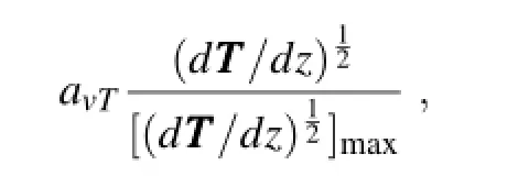
where the constant avTis determined empirically by tuning the assimilation results and setting to 2.7;d TTT /dz is the local vertical temperature gradient at depth z;and[(d TTT /dz)12]maxis the maximum value of(d TTT/dz)12in the water column.The determination of BBBSis analogous to BBBT,except the corresponding constant avSis set equal to 0.6.g( TTT)is a nonlinear T-S relationship function,which is determined from datasets of historical observations.hois the observed value of the sea surface height.σis observational error of the sea surface height,which is set to 6 cm here.The function h(T,S)denotes an observation operator that transforms T and S to the surface dynamic height,which is defined as follows:

where zmis the reference depth,set to 1000 m here.z denotes the vertical coordinate and p denotes the pressure.The functionρ(T,S,p)denotes the sea water state equation for calculating density.ρ0(p)=ρ(0,35,p)is the reference density.More details can be found in Fu et al.(2009a)and Xiao et al.(2008).

Second,the estimated temperature and salinity calculated from the first step are taken as synthetic observations,which are assimilated with the in-situ temperature and salinity observations,such as those from ARGO.The cost function is defined as follows:

where TTT and SSS are the temperature and salinity vectors at the model levels,respectively;and OOOTand OOOSare the observation error covariance matrices of temperature and salinity,respectively.The observation error covariances here are not simple in-situ observation error but include the synthetic observation error and repetitiveness errors of the variability of unresolved smaller scales.Their orders of magnitude are larger than those of the observation errors in the first step.We set the observation errors of temperature and salinity equal to 0.8◦C and 0.1 psu,respectively. HHH is the bilinear interpolation operator that interpolates the model grid points to the observation location. TTTband EEETare the background temperature and its corresponding background error covariance matrix in the horizontal direction,respectively. SSSband EEESare the background salinity and its corresponding error variance matrix,respectively.It should be noted that EEETand EEESare not diagonal matrices.The background error covariance matrix is defined using the Gaussian function as follows:

where A denotes the background error variance of temperature(set to 2.0◦C2)or salinity(set to 0.15 psu2);Δx and Δy are the distances of two horizontal grid points in the zonal and meridional directions,respectively;and Lxand Lyare correlation scales in the zonal and meridional directions,respectively.We take Lx=450 km and Ly=650 km for the temperature,and Lx=420 km and Ly=510 km for the salinity,by tuning the analysis.The detail of the method used to set appropriate values for Lxand Lycan be found in Zhou et al.(2004).

2.3.Ocean observations

In-situtemperatureandsalinity,satellite-SSTand altimeter-derived sea-level anomalies(SLAs)are used for assimilation.The SST observations are from the AVHRR merged product(ftp://eclipse.ncdc.noaa.gov/pub/OI-daily/) created through optimal interpolation(Reynolds et al.,2007). SLAs are from all available satellite altimeters,including T/P, Jason-1/2,ERS-1/2 and Envisat(http://www.aviso.altimetry. fr/en/home.html),which is 0.25◦×0.25◦and a 7-day average gridded dataset.In-situ temperature and salinity are from the GlobalTemperatureand Salinity Profile Project(GTSPP)and ARGO.Quality control is critically important because erroneous values can cause spurious overturning in ocean models.The temperature and salinity profiles used in the study are mainly subject to unified quality control,including a duplicate check(similar position/time check),a depth inversion check,a temperature and salinity valid range check,an excessive gradient check,and a spike value check.The temperature and salinity valid range check applies a gross filter on observed values,which needs to include all of the expected extremes encountered in the oceans(temperature in the range of-2.0◦C to 39.0◦C;salinity in the range of 0.0 to 41.0 psu). The excessive gradient check requires that the ratio of the difference in adjacent values to the difference in the depths is no larger-0.2◦C m-1for temperature and 5.0 psu m-1for salinity.The spike value check requires the test value(α)to be no larger than some pre-defined value:

where V2is the measurement being tested as a spike,and V1and V3are the values above and below the tested layer.Ifαexceeds 6.0 for pressures less than 5000 hPa,orαexceeds 2.0 for pressures less than 5000 hPa,the measurement V2is removed for temperature and salinity.Further details can be found in the ARGO quality control manual,version 2.8(http://www.argodatamgt.org/content/download/15699/ 102401/file/argo-quality-control-manual-version2.8.pdf).

2.4.The operational cycle

The operational BCC GODAS2.0 has been running on a Sunway4000A high-performance computer system at the China Meteorological Administration since 1 April 2014.It runs on six nodes(36 processors)and takes two hours(wall clock)toprocesstheobservationsandthreehourstofinishthe analysis.The data assimilation cycle for the system restarts the model 10 days prior to the most recent time of the NCEP forcing field,while the observations are assimilated within this time window(10 days).The shell scripts controlling the operational run have been implemented to minimize the need for manual operation.A typical daily run starts with the creation of forcing fields for the ocean model.Then,the operational system starts to run after the real-time observations of the SLAs,SST,in-depth temperature and salinity are processed.If the forcing fields are not received by the prescribed time,the model will be forced by the climatological forcing fields.

3.Validation of the operational ocean system

In this study,we evaluate the monthly results from the BCC GODAS2.0 reanalysis for 1990-2011.

3.1.Vertical temperature and salinity errors

The temperature and salinity observations from World Ocean Atlas 2001(WOA01)are used to evaluate the agreement of BCC GODAS2.0 with observations.The vertical profiles of the root-mean-square error(RMSE)of temperature and salinity are shown in Figs.1a and 1b,respectively. Large temperature errors are present mainly in the thermocline,and the errors are largest at a depth of approximately 200 m in the free run.The RMSE of the temperature is reduced at most vertical levels by assimilation.The strong relaxation of the SST constrains the surface temperature variation in the model so that the difference between the results of the free run and the reanalysis results is not obvious in the top layer.The overall RMSE of the temperature is reduced by0.81◦C after the cumulative effect of many assimilation cycles during integration over 22 years.Like the temperature, the RMSE of salinity is reduced by 0.24 psu by assimilation. Note that the improvement can be attributed not only to the assimilation of temperature and salinity but also to the assimilation of the SLA through the dynamic constraints(Yan et al.,2004).

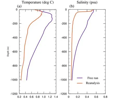
Fig.1.Vertical distribution of RMSE for the temperature and salinity during 1990-2011.The global average statistics are shown for the free run(blue line)and reanalysis(red line).

TheperformanceofBCC GODAS2.0 isfurther evaluated in the tropical Pacific Ocean(30◦S-30◦N,120◦E-70◦W), Indian Ocean(30◦S-30◦N,30◦-120◦E)and Atlantic Ocean (30◦S-30◦N,80◦W-20◦E),separately.Table 1 compares the RMSEs of the free run and the reanalysis.The reduction of RMSE(RRMSE,in%)of the reanalysis relative to the free run is shown as well.The RRMSE is defined in Counillon et al.(2014)as

where RMSEfreeand RMSEreanalysisare the RMSEs of the free run and the reanalysis,respectively.The RMSEs and RRMSEs of temperature(T)and salinity(S)are calculated for surface(0-225 m)and deep(225-1007 m)waters.The RRMSEs of T and S for water depths greater than 1007 m are not examined because the variations of T/S errors with depth are relatively small below 1000 m(as shown in Fig.1). In general,the RRMSE for deep waters is larger than the surface due to less variability than at the surface.The maximum error reductions are achieved in the Atlantic Ocean due to the large errors in the free run.The RRMSEs are greater than 60%at the surface,and greater than 70%in deep waters for both T and S.In the Indian Ocean,the RRMSE is generally larger than 70%for S,while the RRMSE for T is more than 20%.The RRMSE for the Pacific is more than 50%,while for T in the surface layer it is about 33.2%.The relatively low error reduction of RRMSE for T at the surface is mainly caused by the relatively low RMSE in the free run.Overall, the error reductions are significant.

3.2.Mixed layer depth

The mixed layer depth(MLD)is one of the most important quantities of the upper ocean,and its variability strongly influences the physics of the upper ocean and marine biological processes(e.g.,de Boyer Mont´egut et al.,2004; D'Ortenzio et al.,2005;Dong et al.,2007,2009;Ren et al., 2011;Sall´ee et al.,2008;Moore et al.,2013).We estimate the monthly mean MLD from the temperature and salinity based on the density criterion of 0.125(kg m-3),in which the density is supposed to change from that of the ocean surface of 0.125 kg m-3(Levitus,1982).The monthly minimum and maximum MLD for BCC GODAS2.0 and WOA01 are shown in Fig.2.In general,the MLD is deep in winter and shallow in summer for both hemispheres.The minimum MLD in BCC GODAS2.0 is less than 30 m in the midlatitudes.This is consistent with the WOA01 minimum MLD. In the central tropical Pacific,the MLD is 50-60 m,and in the eastern upwelling region the MLD is relatively shallow (＜20 m).A comparison of the minimum MLD with WOA01 illustrates the relatively deep MLD in the Southern Ocean for BCC GODAS2.0.The possible reasons for the differences include deficiencies in model physics and the temporally constant background error covariance in the 3DVAR.It is well known that the Southern Ocean has abundant eddies. The submesoscale eddy-driven restratification of the mixed layer has not been resolved in the model due to the relatively coarse resolution(1◦×1◦)at high latitudes.This is the main contribution to the deeper MLD than those of observations. Another possible reason is that the temporally constant background error covariance in the 3DVAR cannot fully capture the variability of eddies in the Southern Ocean,and thus also cannot simulate eddies well.

A comparison of the maximum MLD highlights the deep mixing in the North Atlantic,consistent with the robust North Atlantic deep water formation.The maximum MLDs in the North Pacific are relatively shallow(＜100 m),also consistent with the lack of deep-water formation there.Homogenous cold and moderately low salinity water is found east of Japan,indicating the formation of the North Pacific Intermediate Water,consistent with Talley(1993).In the Southern Ocean,the observed maximum MLD at 50◦S is approximately 720 m,while the model MLD is over 750 m.Therefore,BCC GODAS2.0 is generally in good agreement with WOA01.

3.3.Sea level variations in the tropical Pacific

Sea level variability is a good indicator of dynamic ocean processes.Some recent studies have noted that the sea level in the tropical Pacific displays significant interannual-todecadal variations in response to climate variability(e.g., Fu et al.,2009b;Merrifield et al.,2012;Qiu and Chen, 2012;Zhuang et al.,2013).To evaluate the model's perfor-mance over the tropical Pacific,empirical orthogonal function(EOF)analysis is applied to low-frequency(period longer than 13 months)SLAs from both altimeter observations and BCC GODAS2.0 simulations.The EOF patterns and the associated principal components(PCs)reflect the spatial and temporal variations,respectively.The first EOF mode of the observed SLA accounts for 54.9%of the total variation,and its EOF-1 shows oppositely signed SLAs in the eastern and western basin(Fig.3a).The EOF-1 of modeled SLAs(Fig.3b),which explains 45.1%of the total variation, generally captures the observed spatial pattern.The modeled PC-1 tracks the observations quite well(Fig.3c;correlation coefficient=0.74,significant at the 95%confidence level), and both show a decadal increasing trend over the past two decades with embedded interannual modulations.A close inspection of the PC-1s reveals that strong sea level oscillations existed in 1994-95,1997-98,2006-07 and 2009-10, indicative of the impacts from El Nin˜o-Southern Oscillation (ENSO)events.

Table 1.The average RMSEs of temperature(T)and salinity(S)estimated from the free run(the reanalysis),and the improvements of the reanalysis relative to the free run(RRMSE,given in%)in the Pacific,Indian and Atlantic Oceans.[0,225]and[225,1007]denote 0-225 m and 225-1007 m depth ranges,respectively.Comparisons are made for the period January 1990 to December 2011.

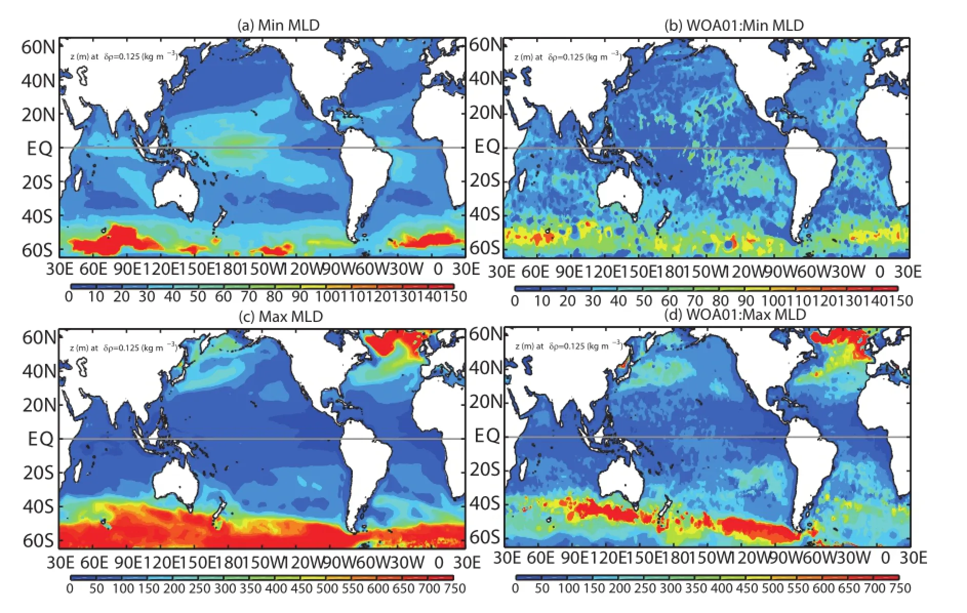
Fig.2.Climatology of the monthly minimum and maximum MLD based on the density criterion 0.125 kg m-3(Levitus,1982)in BCCGODAS2.0 and WOA01.Note that the color scales for the minimum MLD and maximum MLD are different.Panels(a)and(c)are for BCCGODAS2.0 and(b)and(d)are for WOA01.(units:m)

Figure 4 further shows the ability of BCC GODAS2.0 to reproduce sea level trends during 1993-2011.In both BCC GODAS2.0 and observations,the linear sea level trends decrease zonally from west to east,consistent with the results ofthefirstEOFmodesinFig.3.Ingeneral,BCC GODAS2.0 satisfactorily reproduces the sea level rises in the western Pacific,and falls in the eastern Pacific.The most significant risesoccur atthe latitudes of5◦-15◦Nin thenorthwestern Pacific.The zonally opposite sea level trends are mainly caused by the steady intensification of the trade winds across the tropical Pacific that started in the early 1990s(Merrifield and Maltrud,2011;Nidheesh et al.,2013).Recent studies have linked the notable sea level trends,together with the easterly trade intensification,to decadal climate modes,especially the Pacific Decadal Oscillation and the decadal variability of ENSO(Merrifield et al.,2012;Zhang and Church,2012).It isnoteworthythatthemodeledsealeveltrendsinFig.4bhave a basin-mean rate of 1.9 mm yr-1,approximately 25%lower than the mean rate of 2.4 mm yr-1in satellite observations, which is probably because BCC GODAS2.0 does not include the increase in ocean mass resulting from the contributions of ice sheets,melting glaciers and continental waters.

3.4.SST in the tropical Pacific

It is well known that the SST in the tropical Pacific shows significant interannual variability,which greatly influences global climate.In this part,the simulated SST of BCC GODAS2.0 in the tropical Pacific is evaluated.The monthly SSTs from the Hadley Centre Sea Ice and SST dataset(HadISST)on a 1◦×1◦resolution(Rayner et al., 2003),andthe monthlyExtended ReconstructionofSST,version 3b(ERSST.v3b),on a 2◦×2◦resolution(Smith et al., 2008),from 1990 to 2011,are used to validate the analyzed SST.

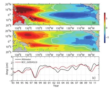
Fig.3.EOF-1 of low-frequency(＞13 months)SLAs derived from(a)altimeter observations and(b)BCC GODAS2.0 simulations for the period 1993-2011.(c)PC-1s of observed and modeled SLA.

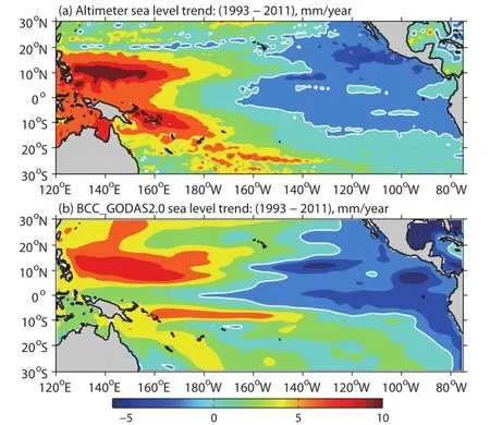
Fig.4.Linear trends of(a)altimetric and(b)BCCGODAS2.0 simulated sea levels during 1993-2011 (units:mm yr-1).

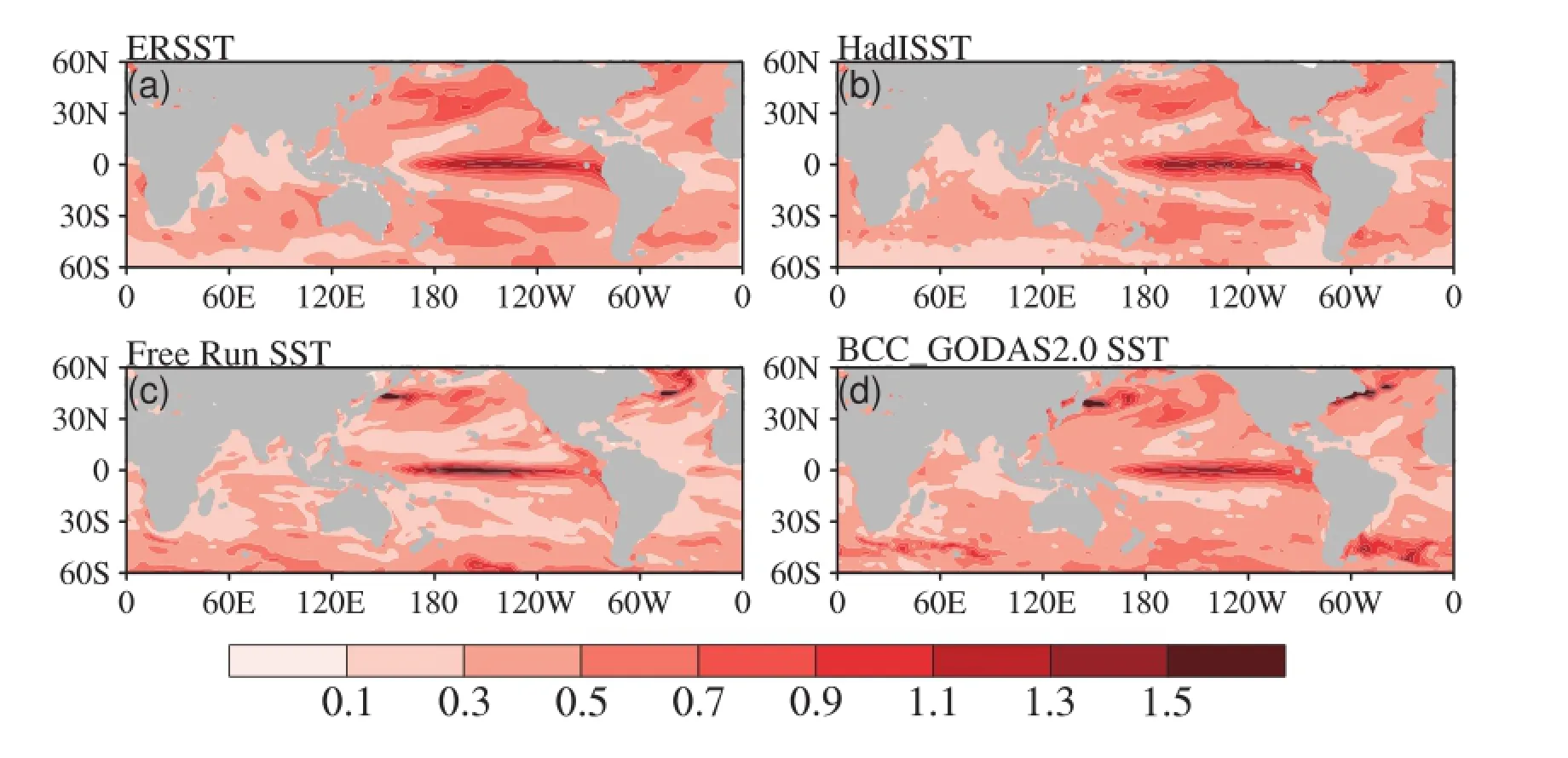
Fig.5.The STD of DJF SST during 1990-2011.Panels(a-d)represent SSTs in ERSST,HadISST,the free run and BCCGODAS2.0,respectively.(units:◦C2).

Spatial distributions of the standard deviation(STD) of the SST in the equatorial Pacific during boreal winter (December-January-February,DJF)are shown in Fig.5.Improvements in the STD of SST by assimilation are mainly located in the tropical Pacific and Atlantic(Figs.5c and d).In the observations(Figs.5a and b),the distributions of the STD are symmetric about the equator,and the maximum centers of the STD are approximately 140◦W.In BCC GODAS2.0, the spatial distributions of the SST STD closely resemble the observations(Fig.5d).However,differences between the observed and simulated SST are found near the east coast of South America,while the SST STDs from BCC GODAS2.0 are weaker than observed,which is probably because the upwelling-favored wind stress used in the model is weaker than in reality,and the model's grid resolution cannot resolve the local bathymetry near the coast of America.

In recent years,two types of El Nin˜o,the canonical El Nin˜o and El Nin˜o Modoki,have been suggested(i.e., Larkin and Harrison,2005;Yu and Kao,2007;Ashok et al.,2007;Kao and Yu,2009;Kug et al.,2009;Wang et al.,2009).The latter is also referred to as the Date Line El Nin˜o(LarkinandHarrison,2005),centralPacificElNin˜o(Yu and Kao,2007),and warm pool El Nin˜o(Kug et al.,2009). The performances of canonical El Nin˜o and Nin˜o Modoki in BCC GODAS2.0 are presented.Here,canonical El Nin˜o is defined by the Nin˜o3 index,which is the area-averaged SST anomalies(SSTA)in the region(5◦S-5◦N,150◦-90◦W). El Nin˜o Modoki is identified by the El Nin˜o Modoki Index (EMI),defined by Ashok et al.(2007)as

EMI=[SSTA]C-0.5×[SSTA]E-0.5×[SSTA]W, where the square brackets with a subscript represent the area-averaged SSTA over the central Pacific region(C) (10◦S-10◦N,165◦E-140◦W),the eastern Pacific region(E) (15◦S-5◦N,110◦-70◦W),and the western Pacific region (W)(10◦S-20◦N,125◦-145◦E),respectively.Figure 6 shows that the changes in both the Nin˜o3 index and the EMI in BCC GODAS2.0 agree well with those from HadISST and ERSST.The correlation coefficients of the two El Nin˜o indices between BCC GODAS2.0 and the two observations exceed 0.9,which are higher than those of the free run (Table 2).The amplitudes of the two El Nin˜o indices in BCC GODAS2.0 show some differences from the observations.The intensities of the Nin˜o3 index in BCC GODAS2.0 are somewhat underestimated.

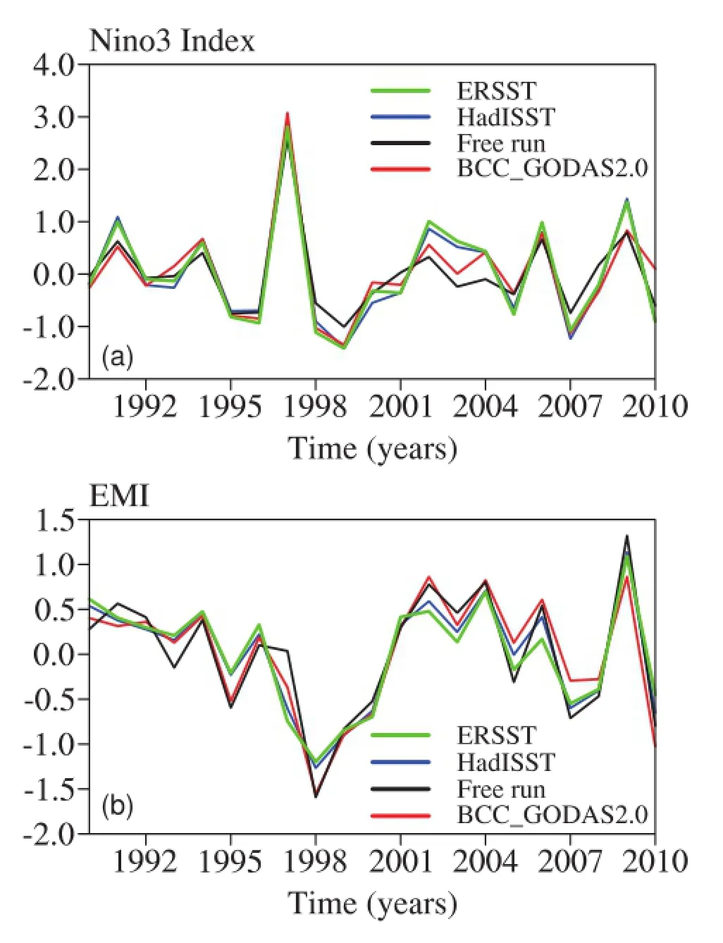
Fig.6.Time series of DJF-mean(a)Nin˜o3 index and(b)EMI during 1990-2011 with ERSST(green line),HadISST(blue line),free run data(black line),and BCC GODAS2.0(red line) (units:◦C).

Table 2.Correlations of BCC GODAS2.0 and the free run SST with the observed SSTs for Nin˜o3 index and EMI.

We next explore the possible reasons why the intensities of the Nin˜o3 index in BCC GODAS2.0 are weaker than those from observations.Figure 7 shows the climatology of the annual SSTs during 1990-2011 in both the simulations and observations.The mean climate state of SSTs in the eastern Pacific in BCC GODAS2.0(Fig.7d)is colder than those from observations(Figs.7a and b).The warmer climate state of SSTs will strengthen the air-sea interaction and increase the amplitudes of the ENSO warm and cold phases(Zhang and Ding,2001;Zhang et al.,2008).The difference in the climatestateofSSTsbetween BCC GODAS2.0andobservations could result in weaker intensities of the Nin˜o3 index in BCC GODAS2.0.As is well known,the two El Nin˜o indices show significant interannual variability.The Nin˜o3 index in the observations has interannual variability with periods of 5 years and 3 years,while the periods of Nin˜o3 index are 4 years in the simulations.The EMI shows the same interannual variability,with periods of 2.5 years in both the observations and simulations(Fig.8).

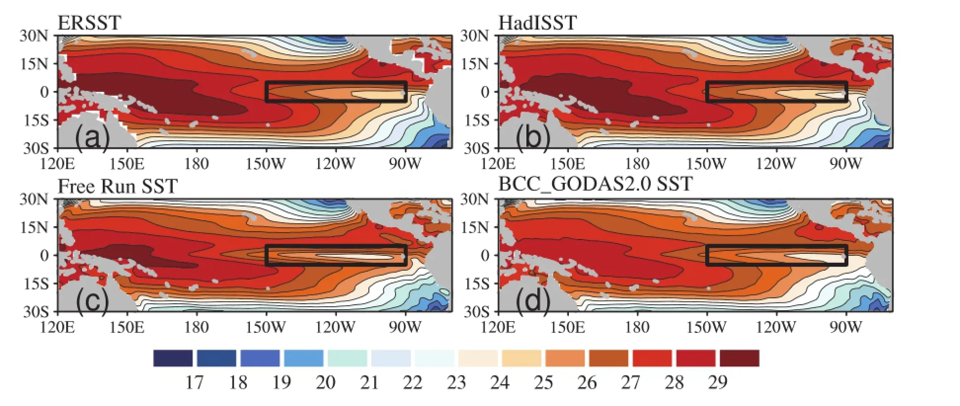
Fig.7.Climatology of annual SSTs during 1990-2011.The black box indicates the region used to calculate Nin˜o3 index.Panels(a-d)represent SSTs in ERSST,HadISST,the free run and BCC GODAS2.0,respectively(units:◦C).

According to their different impacts on rainfall in southern China and typhoon landfall activity,Wang and Wang (2013)separated El Nin˜o Modoki into two subtypes,El Nin˜o Modoki I and II,in which the warm SST anomalies originate from the central tropical Pacific and subtropical northeastern Pacific,respectively.In this study,the simulations of El Nin˜o Modoki I and II in BCC GODAS2.0 are evaluated.Using the classification of Wang and Wang(2013), there are three El Nin˜o Modoki I events(1990/91,1991/92, and 2002/03)and three El Nin˜o Modoki II events(1992/93, 2004/05 and 2009/10).Figure 9 shows the composite SSTAs for El Nin˜o Modoki I and El Nin˜o Modoki II during the developing autumn(September-October-November)from the three datasets of ERSST,HadISST,and BCC GODAS2.0. Similar to those in ERSST and HadISST,the warm SSTAs of El Nin˜o Modoki I in BCC GODAS2.0 are in the central tropical Pacific and are symmetric about the equator.Compared with those in ERSST and HadISST,the warm SSTAs of El Nin˜o Modoki I in BCC GODAS2.0 are weaker,and their area is smaller.The cool SSTAs are observed in the eastern tropical Pacific(Figs.9a-c).For El Nin˜o Modoki II,although the warm SST anomalies of BCC GODAS2.0 show an asymmetric distribution extending and tilting from the subtropical northeastern Pacific to the central equatorial Pacific,as do the observations,their amplitudes are weaker than those in ERSST and HadISST(Figs.9d-f).In addition, the relationships of the Indian Ocean with the two types of El Nin˜o Modoki are reproduced.Wang and Wang(2014)suggested that El Nin˜o Modoki I and II are associated with a positiveandnegativeIODinborealautumn,respectively.Here,a positive IOD means warm/cool SSTAs in the western/eastern tropicalIndianOcean(Sajietal.,1999).InBCC GODAS2.0, the positive and negative IODs are associated with El Nin˜o Modoki I and II,respectively,which is consistent with observations.The amplitude of the positive IOD during El Nin˜o Modoki I in BCC GODAS2.0 is weaker than observed.

4.Summary and conclusions

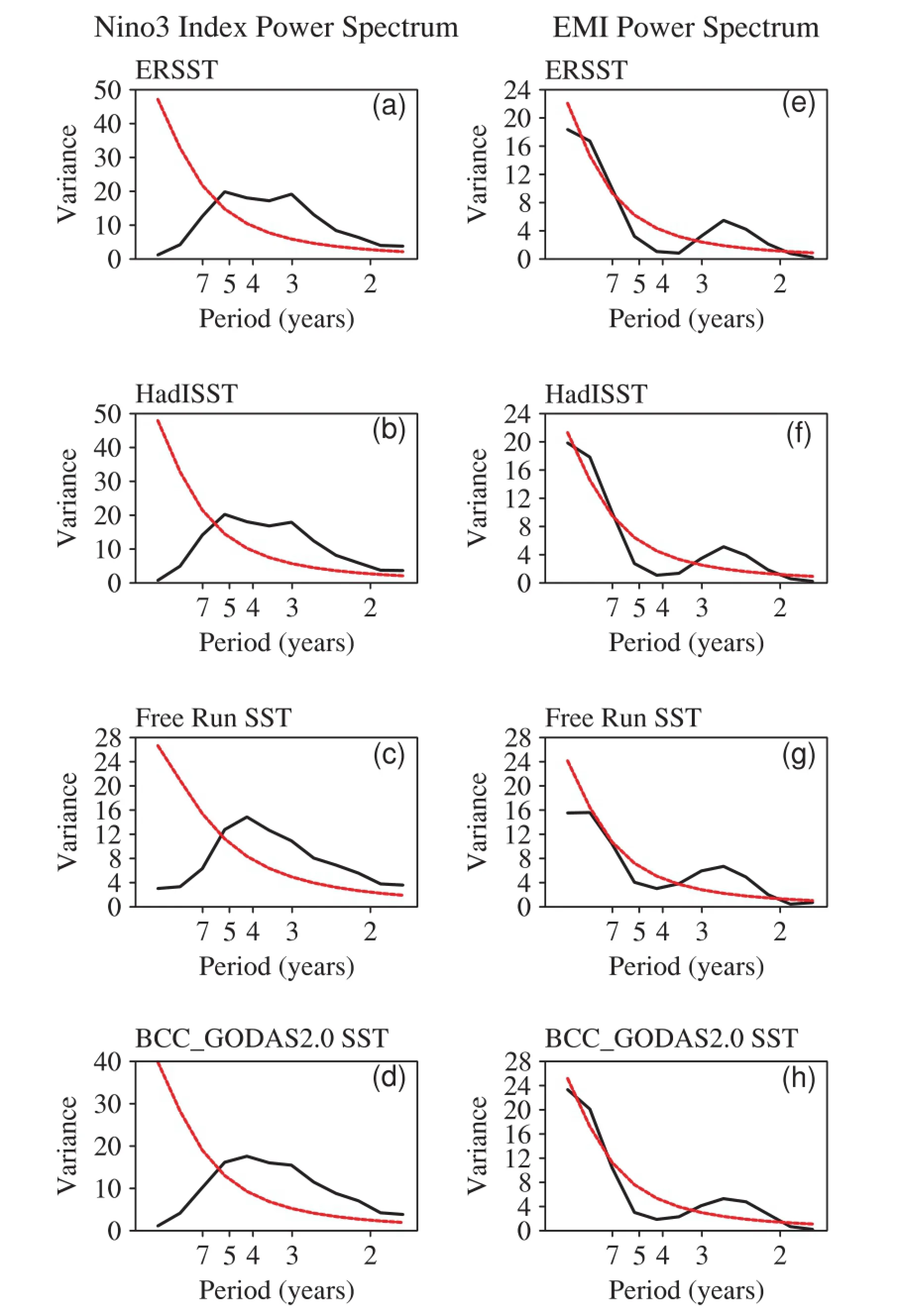
Fig.8.Power spectrum of the monthly(a-d)Nin˜o3 index and(e-h)EMI during 1990-2011.The black curves and red curves represent the calculated spectrum and 90%confidence interval,respectively.The first,second,third and fourth rows represents ERSST,HadISST,the free run and BCC GODAS2.0,respectively.

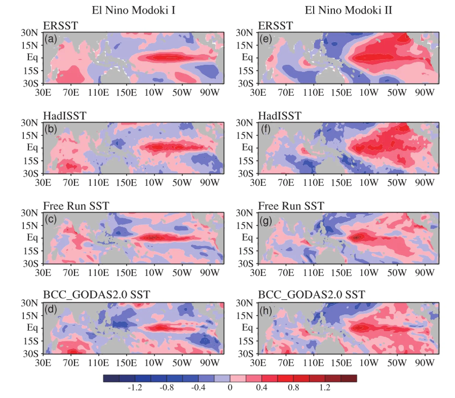
Fig.9.Spatial distributions of composited SSTAs for(a-c)El Nin˜o Modoki I and(d-f)El Nin˜o Modoki II in the boreal autumn(September-November).The first,second,and third row represent ERSST,HadISST and BCC GODAS2.0,respectively.The composites are calculated from three El Nin˜o Modoki I events(1990/91, 1991/92,and 2002/03),and three El Nin˜o Modoki II events(1992/93,2004/05 and 2009/10)(units:◦C).

The second-generation Global Ocean Data Assimilation System of the Beijing Climate Center(BCC GODAS2.0) was implemented in April 2014.The ocean model of BCC GODAS2.0 is MOM4,which adopts tripolar grids to avoid a singularity at the North Pole.An improved 3DVAR scheme is used in BCC GODAS2.0 by adopting a recursive filter to speed up computation.Satellite SLA and SST data and in-situ observations,including ARGO and GTSPP,are assimilated in real time.BCC GODAS2.0 has been run daily in pre-operational mode,driven by six-hourly fluxes from the NCEP.The MLD variation of BCC GODAS2.0 is generally in agreement with that of WOA01.The simulated SST and SSH successfully depict the interannual variability of the tropical Pacific,which has a great impact on the climate of China.It is very important,for the climate monitoring services of the BCC,to evaluate the performance of the tropical Pacific variability in BCC GODAS2.0.In the tropical Pacific,the first EOF and PC of low-frequency SLAs from BCC GODAS2.0 are similar to those from satellite altimeter observations.BCC GODAS2.0 can also satisfactorily reproduce the sea level rises in the western Pacific,and falls in the eastern Pacific.The STD of the SST in BCC GODAS2.0 is similar to those of ERSST and HadISST in the tropical Pacific.The Nin˜o3 index and EMI of BCC GODAS2.0 show highcorrelation(＞0.9)withthoseofERSSTandHadISST.A power spectrum analysis of the monthly averaged SST shows that the Nin˜o3 index and EMI of BCC GODAS2.0 have the most significant periods at approximately 5 and 2.5 years,respectively,which is consistent with ERSST and HadISST. BCC GODAS2.0 can capture the main features of El Nin˜o Modoki I and Modoki II.The performance of the IOD in the BCC GODAS2.0 SST is similar to that observed in the IndianOceanandgenerallyagreeswiththatshowninWangand Wang(2013).The global ocean reanalysis products and realtime assimilation results are being applied in the new generation of the short-term forecast system,BCC CSM1.1.

Acknowledgements.Theauthorswishtothankthetwoanonymous reviewers for their very helpful comments,which helped us to improve the manuscript significantly.Many people have contributed to the development of the BCC GODAS2.0 data assimilation system.We particularly wish to thank Drs.Xianjun XIAO,Zuqiang ZHANG,and Yinhao QIN,for their support and assistance.This study was supported by the National Natural Science Foundation of China(Grant No.41306005),the National Basic Research Program of China(Grant No.2012CB955903)and the CAS/SAFEA International Partnership Program for Creative Research Teams.

REFERENCES

Alves,O.,D.Hudson,M.Balmaseda,and L.Shi,2011:Seasonal and decadal prediction.Operational Oceanography inthe 21st Century,A.Schiller and G.B.Brassington,Eds., Springer,Netherlands,513-542.

Ashok,K.,S.K.Behera,S.A.Rao,H.Y.Weng,and T.Yamagata,2007:El Ni˜no Modoki and its possible teleconnection. J.Geophys.Res.,112,C11007,doi:10.1029/2006JC003798.

Balmaseda,M.A.,K.Mogensen,and A.T.Weaver,2013:Evaluation of the ECMWF ocean reanalysis system ORAS4.Quart. J.Roy.Meteor.Soc.,139,1132-1161.

Behringer,D.W.,M.Ji,and A.Leetmaa,1998:An improved coupled model for ENSO prediction and implications for ocean initialization.Part I:The ocean data assimilation system.Mon.Wea.Rev.,126,1013-1021.

Counillon,F.,I.Bethke,N.Keenlyside,M.Bentsen,L.Bertino, and F.Zheng,2014:Seasonal-to-decadal predictions with the ensemble Kalman filter and the Norwegian Earth System Model:A twin experiment.Tellus A,66,21074.

de Boyer Mont´egut.,C.,G.Madec,A.S.Fischer,A.Lazar,and D. Iudicone,2004:Mixed layer depth over the global ocean:An examination of profile data and a profile-based climatology. J.Geophys.Res.,109,C12003,doi:10.1029/2004JC002378.

Dong,S.F.,S.T.Gille,and J.Sprintall,2007:An assessment of the Southern Ocean mixed layer heat budget.J.Climate,20, 4425-4442,doi:10.1175/JCLI4259.1.

Dong,S.F.,S.L.Garzoli,and M.Baringer,2009:An assessment of the seasonal mixed layer salinity budget in the Southern Ocean.J.Geophys.Res.,114,C12001,doi:10.1029/2008JC 005258.

D'Ortenzio,F.,D.Iudicone,C.de Boyer Montegut,P.Testor, D.Antoine,S.Marullo,R.Santoleri,and G.Madec,2005: Seasonal variability of the mixed layer depth in the Mediterranean Sea as derived from in situ profiles.Geophys.Res. Lett.,32,L12605,doi:10.1029/2005GL022463.

Fu,W.W.,J.Zhu,and C.X.Yan,2009a:A comparison between 3DVAR and EnOI techniques for satellite altimetry data assimilation.Ocean Modelling,26,206-216.

Fu,W.W.,J.Zhu,C.X.Yan,and H.L.Liu,2009b:Toward a global ocean data assimilation system based on ensemble optimum interpolation:Altimetry data assimilation experiment. Ocean Dynamics,59,587-602.

Griffies,S.M.,M.J.Harrison,R.C.Pacanowski,and A.Rosati, 2003:A technical guide to MOM4.NOAA/Geophysical Fluid Dynamics Laboratory,GFDL Ocean Group Tech.Rep. No.5,371 pp.

Griffies,S.M.,and Coauthors,2005:Formulation of an ocean model for global climate simulations.Ocean Science,1,45-79.

Han,G.J.,H.L.Fu,X.F.Zhang,W.Li,X.R.Wu,X.D.Wang, and L.X.Zhang,2013:A global ocean reanalysis product in the China Ocean Reanalysis(CORA)project.Adv.Atmos. Sci.,30,1621-1631,doi:10.1007/s00376-013-2198-9.

Huang,B.Y.,Y.Xue,and D.W.Behringer,2008:Impacts of Argo salinity in NCEP Global Ocean Data Assimilation System: The tropical Indian Ocean.J.Geophys.Res.,113,C08002, doi:10.1029/2007JC004388.

Hunt,B.R.,E.J.Kostelich,and I.Szunyogh,2007:Efficient data assimilation for spatiotemporal chaos:A local ensemble transform Kalman filter.Physica D:Nonlinear Phenomena, 230,112-126.

Kao,H.-Y.,and J.-Y.Yu,2009:Contrasting Eastern-Pacific and Central-Pacific types of ENSO.J.Climate,22,615-632.

Kug,J.-S.,F.-F.Jin,and S.-I.An,2009:Two types of El Ni˜no events:Cold tongue El Ni˜no and warm pool El Ni˜no.J.Climate,22,1499-1515.

Larkin,N.K.,and D.E.Harrison,2005:Global seasonal temperature and precipitation anomalies during El Ni˜no autumn and winter.Geophys.Res.Lett.,32,L16705,doi:10.1029/ 2005GL022860.

Levitus,S.,1982:Climatological atlas of the world ocean.NOAA/ ERL GFDL Professional Paper 13,Princeton,N.J.,173 pp.

Liu,Y.M.,R.H.Zhang,Y.H.Yin,and T.Niu,2005:The application of ARGO data to the global ocean data assimilation operational system of NCC.Acta Meteorologica Sinica,19, 355-365.

Merrifield,M.A.,and M.E.Maltrud,2011:Regional sea level trends due to a Pacific trade wind intensification.Geophys. Res.Lett.,38,L21605,doi:10.1029/2011GL049576.

Merrifield,M.A.,P.R.Thompson,and M.Lander,2012:Multidecadal sea level anomalies and trends in the western tropical Pacific.Geophys.Res.Lett.,39,L13602,doi:10.1029/ 2012GL052032.

Moore,J.K.,K.Lindsay,S.C.Doney,M.C.Long,andK.Misumi, 2013:Marine ecosystem dynamics and biogeochemical cycling in the community earth system model[CESM1(BGC)]: Comparison of the 1990s with the 2090s under the RCP4.5 and RCP8.5 scenarios.J.Climate,26,9291-9312.

Nidheesh,A.G.,M.Lengaigne,J.Vialard,A.S.Unnikrishnan, and H.Dayan,2013:Decadal and long-term sea level variability in the tropical Indo-Pacific Ocean.Climate Dyn.,41, 381-402,doi:10.1007/s00382-012-1463-4.

Qiu,B.,and S.M.Chen,2012:Multidecadal sea level and gyre circulation variability in the Northwestern Tropical Pacific Ocean.J.Phys.Oceanogr.,42,193-206.

Ratheesh,S.,R.Sharma,and S.Basu,2014:An EnOI assimilation of satellite data in an Indian Ocean circulation model.IEEE Transactions on Geoscience and Remote Sensing,52,4106-4111.

Rayner,N.A.,D.E.Parker,E.B.Horton,C.K.Folland,L.V. Alexander,D.P.Rowell,E.C.Kent,and A.Kaplan,2003: Global analyses of sea surface temperature,sea ice,and night marine air temperature since the late nineteenth century.J. Geophys.Res.,108,4407,doi:10.1029/2002JD002670.

Ren,L.,K.Speer,and E.P.Chassignet,2011:The mixed layer salinity budget and sea ice in the Southern Ocean.J.Geophys. Res.,116,C08031,doi:10.1029/2010JC006634.

Reynolds,R.W.,and D.C.Marsico,1993:An improved real-time global sea surface temperature analysis.J.Climate,6,114-119.

Reynolds,R.W.,T.M.Smith,C.Y.Liu,D.B.Chelton,K. S.Casey,and M.G.Schlax,2007:Daily high-resolutionblended analyses for sea surface temperature.J.Climate,20, 5473-5496.

Saji,N.H.,B.N.Goswami,P.N.Vinayachandran,and T.Yamagata,1999:A dipole mode in the tropical Indian Ocean. Nature,401,360-363.

Sakov,P.,F.Counillon,L.Bertino,K.A.Lisæter,P.R.Oke,and A.Korablev,2012:TOPAZ4:An ocean-sea ice data assimilation system for the North Atlantic and Arctic.Ocean Science Discussions,9,1519-1575.

Sall´ee,J.B.,K.Speer,R.Morrow,and R.Lumpkin,2008:An estimate of Lagrangian eddy statistics and diffusion in the mixed layer of the Southern Ocean.J.Mar.Res.,66(4),441-463.

Smith,T.M.,R.W.Reynolds,T.C.Peterson,and J.Lawrimore,2008:Improvements to NOAA's historical merged land-ocean surface temperature analysis(1880-2006).J.Cli-mate,21,2283-2296.

Talley,L.D.,1993:Distribution and formation of North Pacific intermediate water.J.Phys.Oceanogr.,23,517-537.

Wang,C.Z.,and X.Wang,2013:Classifying El Ni˜no Modoki I and II by different impacts on rainfall in Southern China and typhoon tracks.J.Climate,26,1322-1338.

Wang,D.X.,Y.H.Qin,X.J.Xiao,Z.Q.Zhang,and X.Y.Wu, 2012a:El Ni˜no and El Ni˜no Modoki variability based on a new ocean reanalysis.Ocean Dynamics,62,1311-1322.

Wang,D.X.,Y.H.Qin,X.J.Xiao,Z.Q.Zhang,and F.M.Wu, 2012b:Preliminary results of a new global ocean reanalysis. Chinese Science Bulletin,57,3509-3517.

Wang,X.,D.Wang,and W.Zhou,2009:Decadal variability of twentieth-century El Ni˜no and La Ni˜na occurrence from observations and IPCC AR4 coupled models.Geophysical research letters,36,L11701.

Wang,X.,and C.Z.Wang,2014:Different impacts of various El Ni˜no events on the Indian Ocean Dipole.Climate Dyn.,42, 991-1005.

Wu,T.W.,and Coauthors,2013:Progress in developing the shortrange operational climate prediction system of China national climate center.Journal of Applied Meteorological Science, 24,533-543.(in Chinese)

Wu,T.W.,and Coauthors,2014:An overviewof BCC climate system model development and application for climate change studies.Journal of Meteorological Research,28,34-56.

Xiao,X.J.,D.X.Wang,C.X.Yan,and J.Zhu,2008:Evaluation of a 3dVAR system for the South China Sea.Progress in Natural Science,18,547-554.

Xue,Y.,B.Y.Huang,Z.-Z.Hu,A.Kumar,C.H.Wen,D. Behringer,and S.Nadiga,2011:An assessment of oceanic variability in the NCEP climate forecast system reanalysis. Climate Dyn.,37,2511-2539.

Yan,C.X.,J.Zhu,R.F.Li,and G.Q.Zhou,2004:Roles of vertical correlations of background error and T-S relations in estimation of temperature and salinity profiles from sea surface dynamic height.J.Geophys.Res.,109,C08010,doi: 10.1029/2003JC002224.

Yu,J.-Y.,and H.-Y.Kao,2007:Decadal changes of ENSO persistence barrier in SST and ocean heat content indices:1958-2001.J.Geophys.Res.,112,D13106,doi:10.1029/2006JD 007654.

Zhang,Q.,and Y.-H.Ding,2001:Decadal climate change and ENSO cycle.Acta Meteorologica Sinica,59,157-172.(in Chinese)

Zhang,Q.,Y.Guan,and H.-J.Yang,2008:ENSO amplitude change in observation and coupled models.Adv.Atmos.Sci., 25,361-366,doi:10.1007/s00376-008-0361-5.

Zhang,X.B.,and J.A.Church,2012:Sea level trends,interannual and decadal variability in the Pacific Ocean.Geophys. Res.Lett.,39,L21701,doi:10.1029/2012GL053240.

Zheng,F.,and J.Zhu,2015:Roles of initial ocean surface and subsurface states on successfully predicting 2006-2007 El Ni˜no with an intermediate coupled model.Ocean Science,11,187-194,doi:10.5194/os-11-187-2015.

Zheng,F.,J.Zhu,H.Wang,and R.-H.Zhang,2009:Ensemble hindcasts of ENSO events over the past 120 years using a large number of ensembles.Adv.Atmos.Sci.,26(2),359-372, doi:10.1007/s00376-009-0359-7.

Zhou,G.Q.,W.W.Fu,J.Zhu,and H.J.Wang,2004:The impact of location-dependent correlation scales in ocean data assimilation.Geophys.Res.Lett.,31,L21306,doi:10.1029/2004 GL020579.

Zhuang,W.,B.Qiu,and Y.Du,2013:Low-frequency western Pacific Ocean sea level and circulation changes due to the connectivity of the Philippine Archipelago.J.Geophys.Res., 118,6759-6773.

Zhou,W.,M.Y.Chen,W.Zhuang,F.H.Xu,F.Zheng,T.W.Wu,and X.Wang,2016:Evaluation of the tropical variability from the Beijing Climate Center's real-time operational Global Ocean Data Assimilation System.Adv.Atmos. Sci.,33(2),208-220,

10.1007/s00376-015-4282-9.

28 April 2015;revised 26 July 2015;accepted 31 July 2015)

∗Wei ZHOU

Email:zhouwei@cma.gov.cn