A Microscale Model for Air Pollutant Dispersion Simulation in Urban Areas: Presentation of the Model and Performance over a Single Building
2016-11-25NingZHANGYunsongDUandShiguangMIAO
Ning ZHANG,Yunsong DU,and Shiguang MIAO
1Institute for Climate and Global Change Research and School of Atmospheric Sciences,Nanjing University,Nanjing 210093
2Sichuan Environmental Monitoring Center,Chengdu 610091
3Institute of Urban Meteorology,China Meteorological Administration,Beijing 100089
A Microscale Model for Air Pollutant Dispersion Simulation in Urban Areas: Presentation of the Model and Performance over a Single Building
Ning ZHANG∗1,Yunsong DU1,2,and Shiguang MIAO3
1Institute for Climate and Global Change Research and School of Atmospheric Sciences,Nanjing University,Nanjing 210093
2Sichuan Environmental Monitoring Center,Chengdu 610091
3Institute of Urban Meteorology,China Meteorological Administration,Beijing 100089
A microscale air pollutant dispersion model system is developed for emergency response purposes.The model includes a diagnostic wind field model to simulate the wind field and a random-walk air pollutant dispersion model to simulate the pollutant concentration through consideration of the influence of urban buildings.Numerical experiments are designed to evaluate the model's performance,using CEDVAL(Compilation of Experimental Data for Validation of Microscale Dispersion Models)wind tunnel experiment data,including wind fields and air pollutant dispersion around a single building.The results show that the wind model can reproduce the vortexes triggered by urban buildings and the dispersion model simulates the pollutant concentration around buildings well.Typically,the simulation errors come from the determination of the key zones around a building or building cluster.This model has the potential for multiple applications;for example,the prediction of air pollutant dispersion and the evaluation of environmental impacts in emergency situations;urban planning scenarios; and the assessment of microscale air quality in urban areas.
numerical model,urban air pollution,air pollutant dispersion,emergency response model
1.Introduction
Urbanization is a worldwide process through which human beings change the natural world.The natural/vegetated land surface is converted to an urban land surface composed of buildings.Large amounts of material and energy are consumed in urban areas and pollutants and waste heat are released as a result.With urbanization taking place all around the world,many related environmental problems occur over urban areas from the regional to the building scale(e.g.Britter and Hanna,2003;Britter et al.,2003;Ren et al.,2011). Air pollutant dispersion at the microscale is very important because it is closely related to the comfort and health of residents in populated urban areas.However,the characteristics of pollutant dispersion in urban areas at the local scale and microscale is complicated because of the complex wind field disturbed by buildings of various shapes(Walton et al.,2002; Hanna et al.,2003;Shi et al.,2008;Xie et al.,2008;Boppana et al.,2010;Fujiwara et al.,2011;Gu et al.,2011;Zhang et al.,2011;Chung and Liu,2013;Perret and Savory,2013). The SIRANE model(Soulhac et al.,2011,2012)improvedthe conventional Gaussian model by integrating a box model for street canyons and considering the fluxes at street intersections.
Numerical simulation is an important method widely used for the urban atmospheric environment and many models have been developed for microscale pollutant dispersion. The“urbanized”Gaussian model is a conventional method that tries to consider the impact of buildings by modifying the horizontal and vertical diffusion parameters(McElroy,1969; Hanna,1971).This method works well when the building density is quite low(Hanna et al.,2003;Luhar et al.,2006; Venkatram and Princevac,2008),but fails in areas with highrise buildings.
The abilities of computational fluid dynamics(CFD) methods(e.g.,large-eddy simulation,direct numerical simulation)are similar in terms of their representation of the wind flow characteristics around buildings and urban canyons(Cai, 2000;WaltonandCheng,2002;Waltonetal.,2002;Caietal., 2004;Meroney,2006,2008;Shi et al.,2008;Gousseau et al., 2011;Zhang et al.,2011;Aumond et al.,2012;Hertwig et al., 2012;Inagaki et al.,2012;Saneinejad et al.,2012;Michioka et al.,2013).However,such methods are usually quite expensive computationally,and less effective in an emergency response setting.
©Institute of Atmospheric Physics/Chinese Academy of Sciences,and Science Press and Springer-Verlag Berlin Heidelberg 2016
Regarding emergency responses at the urban neighborhood scale(e.g.,toxic gas leakages,airborne aerosol emissions),information on air pollutant dispersion and evaluations of the likely harm should be supported over a very short timeframe(about 10-30 minutes)for a decision to made(van de Walle and Turoff,2008).A fast method is needed to simulate the wind flow/air dispersion around building clusters with relatively high accuracy and less computational cost. A few models have been developed for this purpose,e.g., QUIC(The Quick Urban and Industrial Complex dispersion model system)developed by the Los Alamos National Laboratory(www.lanl.gov/projects/quic/index.shtml)(Singh et al.,2008).Inthispaper,anurbanmicroscaleairpollutiondispersion simulation model(hereafter,UMAPS)is established and evaluated with wind tunnel experiments.
2.The model
The model(UMAPS)is a building-resolved air pollutant dispersion model system,which includes a diagnosis model for wind fields around urban buildings(Wind Information Field Fast Analysis Model,WIFFA)and a random-walk air pollutant dispersion model(Nanjing University Random-Walk Dispersion Model,NJU-RWM)to simulate the pollutant transport in urban canopies or canyons.
2.1.WIFFA
WIFFA is responsible for calculating the wind fields for the dispersion model.WIFFA includes two modules,a firstguess wind field interpolation model and a mass conservation wind model.The first-guess wind field interpolation model supplies the initial conditions for the mass conservation wind model,based on building morphology information and background wind speed/direction.The mass conservation model calculates a more realistic wind field based on the mass continuity equation.
Theimpactofthebuildingisconsideredviathemethodof the QUICmodel(http://www.lanl.gov/projects/quic/quicurb. shtml),in which the wind field around a building is characterized by several key zones,including the upwind displacement zone,the upwind cavity,the leeside cavity,the wake zone,and the rooftop recirculation zone due to the prevailing wind direction,and the reference wind speed is used for the interpolation in different zones.Both the wind fields in the leeside cavity and wake zone are determined by the method of R¨ockle(1990).Wind fields in the upwind displacement zone and upwind cavity are estimated by the method of Bagal et al.(2004a,b),and the interpolation method of Pol et al.(2006)is used for the rooftop recirculation zone.
The interaction among buildings causes the wind flow in a street canyon to be more complicated than around a single building.Oke(1988)classified the wind flow in a street canyon into three types:isolated roughness flow,wake interference flow,and skimming flow.For the isolated roughness flow,the interpolation method for a single building is used in our model.For the skimming flow and the wake interference flow,the method of Kaplan and Dinar(1996)is used.
The shapes of buildings in an urban area in the real world are far more complicated than a cube or rectangle.In UMAPS,all buildings are simplified to be a rectangle characterized by the maximum building length,width and height,to take advantage of the idealized interpolation schemes introduced above.Also,all the above interpolation methods work under the assumption that the inlet wind flow is perpendicular to the building wall.When the inlet wind flow is not perpendicular to the building wall,an adjustment is made using the method of Kaplan and Dinar(1996).
Two schemes are used for wind profile interpolation in WIFFA.The power profile method(R¨ockle,1990)is used as the QUICK-URB model when the building coverage is low (buildingscoveringafractionlessthanorequalto35%,inthe current experiments)and the buildings distribution is sparse. The interpolation equation is as follows:

where u0(zref)is the reference wind speed,zrefis the reference height,p is the power index,z is the vertical height, and u0(z)is the interpolated wind speed at the height of z. When the building intensity is high(coverage greater than 35%),the urban canopy profile method(Macdonald,2000) is used,because the power method usually overestimates the wind speed below the height of buildings.The equation of the urban canopy profile is as follows:

where Hcanis the height of the canopy(in this paper,its value is set to the average building height of the whole simulation domain),ucanisthewindspeedatthetopoftheurbancanopy, d isthedisplacementheight(inthispaper,itissetas0.7Hcan), z0istheroughnesslength(about0.1-0.2Hcan),andα(z)isthe decay exponent,which is a function of z and the building intensityofthehorizontalsectionattheheightofz(Macdonald, 2000).
After the first-guess interpolation,an initial wind field is created and the wind speed at the grids that are inside the buildings are set to zero,but the interaction of the wind fields between“building-impact”grids and background grids are not considered.The mass conservation equation is taken into account to obtain a more realistic wind field from the first-guess result.Mass-conservation wind models have been widely used to simulate the wind field over complex terrain for air pollutant dispersion(Goodin et al.,1980;Ross et al., 1988;Jiang et al.,2001).The model used in UMAPS was originally developed by Jiang et al.(2001),and the building influence is considered as a very sharp topography.
2.2.NJU-RWM
The random-walk method is widely used in air pollutant dispersion simulations,which tracks tracer particles through advection by the mean wind field and diffusion by atmospheric turbulence.The turbulence movement is estimated by calculating the probability distribution of particle movement, which is simulated by a random number.A large number of particles are used to statistically simulate the distribution of pollutant mass,and concentrations are calculated by the distribution of tracer particles.This method is also widely used in urban dispersion simulations(e.g.,Delay and Bodin,2001; Wang and Mu,2011).NJU-RWM is a random-walk model developed by Jiang et al.(1999).The model has been modified to consider the influence of buildings and verified by Zhang and Jiang(2006).
3.Wind tunnel experiment database and numerical case design
3.1.Wind tunnel experiment database and numerical experiment settings
The CEDVAL(Compilation of Experimental Data for Validation of Microscale Dispersion Models,http://www. mi.uni-hamburg.de/CEDVAL ValidationData.427.0.html) database is selected for the model evaluation in this paper. The CEDVAL experiments were carried out at Hamburg University,and include mean wind field,turbulence,and air pollutant concentration measurements for single buildings and building clusters.This database is widely used for the development and evaluation of microscale numerical models (Di Sabatino et al.,2008;Castelli and Reisin,2011;Parente et al.,2011;Vardoulakis et al.,2011).
The A1-1 and A1-5 wind tunnel experiments in CEDVAL are used to evaluate the performance of the wind field simulation by UMAPS around a single building;the numerical experiments are named SA1-1 and SA1-5,respectively.The model uses Cartesian coordinates and a regular cubic grid is deployed.The horizontal simulation domain is 450 m in the inlet wind velocity direction(x direction),200 m in the crosswind direction(y direction),and 100 m in the vertical direction(z direction).The grid resolution is 1 m.The inlet wind profile for the numerical experiments is set as the same power-exponent profiles as in the wind tunnel setting, as follows:

where Hrefis the reference height,which is 100 m in A1-1/SA1-1 and 125 m in A1-5/SA1-5;Urefis the inlet wind speed at the height of Href,which is 6.0 m s-1in A1-1/SA1-1 and 5.85 m s-1in A1-5;and p is the power exponent parameter,which is 0.21 in all experiments.
In the A1-5 wind tunnel experiment,four sources are placed on the ground near the leeside wall of the building.The pollutant concentration observations are represented by dimensionless concentration,defined as K=cm×Uref× H2/Qs,where cmis the pollutant concentration,Urefis the reference wind speed,as in Eq.(3),and Qsis the total mass of pollutant release.H is the building height.In the numerical experiments,the wind field is simulated by WIFFA,and then NJU-RWM is deployed to simulate the air pollutant dispersion.A total of 400 000 particles are released to simulate the pollutant dispersion in NJU-RWM.
3.2.Performance evaluation
To evaluate the performance of the model system,the following statistical parameters are employed:
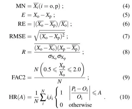
Here,Xois the observed variable(wind speed,wind components,or pollutant concentration)and Xpis the respective modeled one.MN is the mean value;E is the mean error between simulations and observations,RE is the relative simulation error;RMSE is the root-mean-square error;R is the correlation coefficient;FAC2 is the factor of two of observations;N(0.5≤Xp/Xo≤2.0)is the data number under the condition(0.5≤Xp/Xo≤2.0);N is the total data number; HR is the hit rate;and A is the threshold value of relative error.
4.Results
Thesimulatedresultsarefirstinterpolatedtothemeasurement points of the wind tunnel experiments for the evaluation.The CEDVAL A1-1 and A1-5 experiments relate to the wind fields and pollution dispersion around a single building; the building size is 20 m in the x direction,30 m in the y direction,and the height is 35 m.The simulation results show that UMAPS captures the wind field structures well compared to the wind tunnel experiments.In both the numerical simulations and wind tunnel observations,the displacement point occurs at about x/H=-1.0 to 1.3,and the stagnation point occurs at z/H=0.7.The reattachment point is at the location of x/H=2.2,and the wind speed in the windward vortex is less than 2.0 m s-1(Fig.1).These results are consistent with the simulations reported in Singh et al.(2008). The vertical leeside cavity vortex and the horizontal doubleeyed vortex are represented well in the simulations(Fig.2).A clockwise vortex appears and the vortex eye occurs at the location of(x/H=0.9 and z/H=0.9)in the vertical section. In the horizontal section,the eyes of the symmetric vortexes occur at(x/H=0.7,y/H=±0.6),compared to(x/H=0.7, y/H=±0.4)inthewindtunnelexperiments.Thewindspeed in the leeside cavity is less than 1.5 m s-1,and the wind speed increases to 3.0 m s-1at heights greater than the leeside cavity.
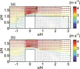
Fig.1.The wind velocities at the crossing section y/H=0: (a)CEDVAL observations;(b)numerical simulations.A:wind cavity;B:roof-top circulation;C:leeside cavity and wake zone.
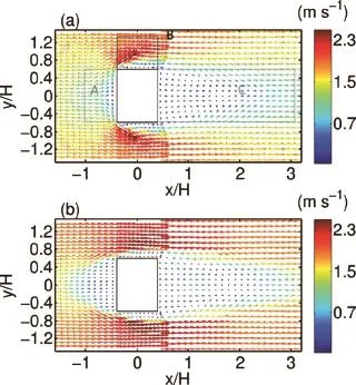
Fig.2.The wind velocities at the crossing section of z/H= 0.28:(a)CEDVAL observations;(b)numerical simulations.A: wind cavity;B:lateral wall zone;C:leeside cavity and wake zone.
To analyze the model performance in a more detailed way,the evaluation parameters are calculated not only for the whole y/H=0 section,but also for the key zones,including the windward zone,the leeside zone,and the rooftop zone, as shown in Fig.1.The model simulation for this section is good,with a mean RE of 6.4%and R=0.96.Table 1 lists the statistical parameters of wind speed in different zones, and shows that the model performs better in the windward zone and rooftop zone,as compared to the leeside zone.The RE of the leeside zone is 21.3%,compared to a 5.4%in the windward zone and 3.7%in the rooftop zone.Figure 3 illustrates the vertical profile of u and w at different locations in the y/H=0 section.The simulation represents the blocking of wind by the building,the upward motion before the building,and the downward motion behind the building.For the y/H=0 section,the model overestimates the total wind speed and u component slightly,with a maximum E of 0.34 m s-1.The larger simulation errors of u occur in the leeside profiles at the level between z/H=0.8 and 1.2.This area is the transition area from the leeside cavity and wake zone to the background flow,and the model describes a sharper transition compared to the tunnel experiment.
For the wind tunnel observations and numerical simulations of wind fields in the z/H=0.28 section(Fig.2),the RE of the whole section is 1.4%and R=0.91.Three key zones are again selected for a more detailed evaluation(the windward zone,leeside zone and lateral-wall zone),as shown in Fig.2,and the related evaluation parameters are listed in Table 2.The largest simulation error happens in the windward area,where the average wind speed of the wind tunnel experiment is 2.55 m s-1,while that of the simulation is 1.88 m s-1.The RE is 25.1%,compared to 5.2%in the leeside zone, 4.9%in the lateral-wall zone,and 1.4%for the whole section.Figure 4 illustrates the horizontal profile of u and v at different locations at x/H=-1.6,-1,-0.5,0,0.5,1,2,and 3.The modeled horizontal wind components are consistent with the simulations.The largest error of u is of 0.25 m s-1, which occurs at x/H=3.0;and the largest RMSEs of u are about 0.63 m s-1and 0.61 m s-1,occurring at x/H=-1.0 and x/H=3.0,where the frontal eddy and leeside vortex occur,respectively.The largest MD of v is only 0.01 m s-1, but with a large RMSE of about 1.17 m s-1,which happens at x/H=-0.5.The errors of the windward zone come fromthe overestimation of the area of the frontal eddy,based on R¨ockle(1990).

Table 1.Comparison of measurements and simulations in section y/H=0 in experiment SA1-1.
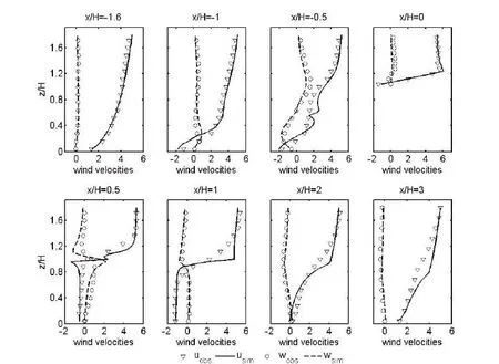
Fig.3.The vertical profiles of wind components(u and w)at the plane of y/H=0 in A1-1 and SA1-1.

Table 2.Comparison of measurements and simulations in section z/H=0.28 in experiment A1-1 and SA1-H1.
Figures 5 and 6 illustrate the horizontal distribution of the dimensionless concentration K in the horizontal sections of z/H=0.08,z/H=0.28 and y/H=0 in A1-5 and SA1-5.High concentration occurs in the leeside cavity circulation and lateral-wall-side circulation,and the maximum concentration appears in these area instead of the middle axis of the circulations.This is because the vortex structure in the leeside cavity may cause the pollutant to be concentrated and a flow reversal in the background wind direction would bring the pollutant windward into the lateral-wall-side circulations. Behind the leeside cavity,the concentration decreases with distance dramatically,and the decreasing trend in numerical simulations is higher than that in the wind tunnel experiments.
In the wind tunnel experiments and numerical simulation results,the pollutant concentration in the z/H=0.08 section is higher than that in the z/H=0.28 section because the pollutant source is on the ground.The maximum of the dimensionless concentration K is 70.4 for z/H=0.08 and 21.5 for z/H=0.28 in the wind tunnel experiment,but 92.7 and 32.1 in the numerical simulations.This demonstrates the model overestimates the peak value of the pollutant concentration but underestimates the dispersion area.The maximum appears just at the corner of the leeside wall and lateral side wall in the wind tunnel experiment,but it appears at the location just behind the leeside wall in the simulation.This is due to the overestimation of the lateral-wall-side circulations in WIFFA.
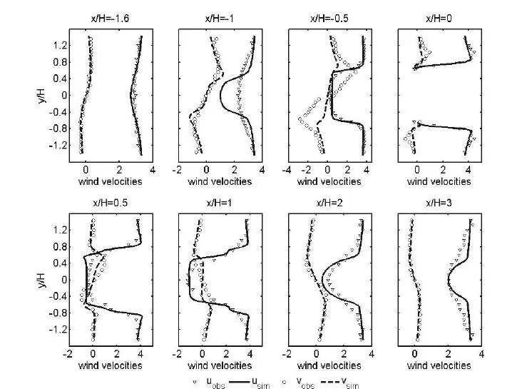
Fig.4.The horizontal profiles of wind components(u and v)at the plane of z/H=0.28 in A1-1 and SA1-1.
For the results of the vertical section,both the wind tunnel experiment and the numerical simulations show that high concentration occurs near the leeside wall area in the leeside cavity.Under the combined influence of the leeside cavity vortex and rooftop vortex,high concentration also occurs over the building roof.The largest simulation error appears in the transition zone from the leeside cavity vortex to the background wind flow.In this area,the model underestimates the pollutant concentration due to the overestimation of wind speed.
In the y/H=0 section,both the wind tunnel experiment and numerical simulation show the highest concentration appearing in the ground corner of the leeside wall,with the maximum being 66.7 in the wind tunnel experiment and 62.5 in the numerical simulation.On the roof top level,both in the wind tunnel experiment and the numerical simulation,there is a high concentration at the leeside corner,with a maximum K of 1.66 in the experiments and 0.82 in the numerical simulation results.The numerical simulation shows a low pollutant concentration at the lowest model layer(at the height of 1 m).This is because,in the RWM,the tracer particle will bounce back when it encounters the surface or building walls. Such an influence can increase when the vertical resolution is coarse and add several buffer levels between the ground and the lowest layer.
Table 3 shows the evaluation parameters for the dimensionless pollutant concentration.The model slightly underestimates the concentration for all three sections.The RE is 10.8%for the vertical section and 35.1%for the horizontal section.However,the model represents the horizontal concentration distribution better;the R values of section z/H=0.08 and 0.28 are 0.77 and 0.70,respectively,which are greater than the value of 0.60 for section y/H=0.For all sections,the FAC2s and HRs are greater than 50%and60%,which have been used as threshold values for model evaluations in previous research(e.g.,Vardoulakis et al., 2011;Parente et al.,2011).This means that the model is reliable for pollutant dispersion simulation.

Table 3.Comparison of dimensionless concentration in A1-5 and SA1-5.
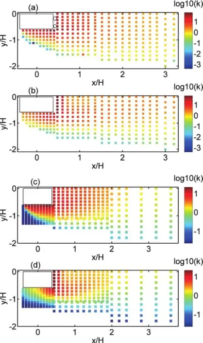
Fig.5.The dimensionless pollutant concentration in the horizontal section:(a)wind tunnel experiment result in A1-5 at z/H=0.08(the circles indicate the locations of sources);(b) numerical simulation result in SA1-5 at z/H=0.08;(c)wind tunnel experiment result in A1-5 at z/H=0.28;(d)numerical simulation result in SA1-5 at z/H=0.28.
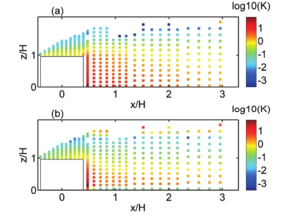
Fig.6.The dimensionless pollutant concentrationy in the vertical section y/H=0:(a)wind tunnel experiment resHult in A1-5;(b) numerical simulation result in SA1-5.
5.Summary
UMAPSisamicroscaleairpollutantmodelsystemdeveloped for air pollutant dispersion simulation under emergency release conditions.It includes a diagnostic wind field model (WIFFA)and a random-walk air pollutant dispersion model (NJU-RWM)to simulate the wind fields and pollutant concentration in detail,through consideration of the influence of urban buildings.The wind field model is composed of two parts:an interpolation model,to obtain the first-guess fields of different zones around a building or street canyon;and a mass conservation wind model,to obtain a detailed wind field in the whole simulation domain.NJU-RWM reproduces the air pollutant dispersion by releasing tracer particles.
The CEDVAL database is used to evaluate the model's performance.The wind field and pollutant dispersion experiments around a single building are used to evaluate the simulation results.The simulation error,relative error,correlation coefficient,and root-square simulation error are used to evaluate the model's performance.The comparisons show that the model can reproduce the wind fields and pollutant dispersion around a typical rectangular building.Generally,the model overestimates the wind speed and underestimates the pollutant concentration.The largest uncertainty relates to the determination of the size of the key zones and the simplification of the complex building shape.This indicates that the definition parameters of the key zones around the building are important for model performance.Evaluations of the model's performance over more complex and realistic conditions will be carried out in the next stage of model development.
UMAPS is a simple and fast model,which does not demand much computational resource and can work on a personal computer.It also works well with operational meteorological observations or numerical weather predictions.This model has the potential for multiple applications;for example,to predict air pollutant dispersion and evaluate environmental impacts in emergency response situations,in urban planning scenarios,and for assessing microscale air quality in urban areas.
Acknowledgements.This work was supported by the National Natural Science Foundation of China(Grant No.41375014),the National Basic Research Program of China(Grant No.2011CB 952002)and Jiangsu Collaborative Innovation Center for Climate Change,China.
REFERENCES
Aumond,P.,V.Masson,C.Lac,B.Gauvreau,S.Dupont,and M.Berengier,2012:Including the drag effects of canopies: Real case large-eddy simulation studies.Bound.-Layer Me-teor.,146,65-80.
Bagal,N.L.,E.R.Pardyjak,and M.J.Brown,2004a:Improved upwind cavity parameterizations for a fast response urban wind model.Proc.84th Annual Meeting Symp.Planning, Nowcasting and Forecasting Urban Zone,Seattle,WA,USA, American Meteorological Society,5 pp.
Bagal,N.L.,B.Singh,E.R.Pardyjak,and M.J.Brown,2004b: Implementation of rooftop recirculation parameterization into the QUIC fast response urban wind model.Proc.5th AMS Urban Environ.Symp.Conf.,Vancouver,B.C.,American Meteorological Society.27 pp.
Boppana,V.B.L.,Z.T.Xie,and I.P.Castro,2010:Large-eddy simulation of dispersion from surface sources in arrays of obstacles.Bound.-Layer Meteor.,135,433-454.
Britter,R.E.,and S.R.Hanna,2003:Flow and dispersion in urban areas.Annual Review of Fluid Mechanics,35,469-496.
Britter,R.E.,S.R.Hanna,G.A.Briggs,and A.Robins,2003: Short-range vertical dispersion from a ground level source in a turbulent boundary layer.Atmos.Environ.,37,3885-3894.
Cai,X.M.,2000:Dispersion of a passive plume in an idealised urban convective boundary layer:A large-eddy simulation. Atmos.Environ.,34,61-72.
Cai,X.M.,M.Nasrullah,and Y.Huang,2004:Fumigation of pollutants into a growing convective boundary layer over an inhomogeneous surface:A large eddy simulation.Atmos.Environ.,38,3605-3616.
Castelli,S.T.,and T.G.Reisin,2011:Application of a modified version of RAMS model to simulate the flow and turbulence in the presence of buildings:The MUST COST732 exercise. International Journal of Environment and Pollution,44,394-402.
Chung,T.N.H.,andC.H.Liu,2013:Onthemechanismofairpollutantremovalintwo-dimensionalidealizedstreetcanyons:A large-eddy simulation approach.Bound.-Layer Meteor.,148, 241-253.
Delay,F.,and J.Bodin,2001:Time domain random walk method to simulate transport by advection-dispersion and matrix diffusion in fracture networks.Geophys.Res.Lett.,28,4051-4054.
Di Sabatino,S.,E.Solazzo,P.Paradisi,and R.Britter,2008:A simple model for spatially-averaged wind profiles within and above an urban canopy.Bound.-Layer Meteor.,127,131-151. Fujiwara,C.,K.Yamashita,M.Nakanishi,and Y.Fujiyoshi,2011: Dust devil-like vortices in an urban area detected by a 3D scanning Doppler lidar.Journal of Applied Meteorology and Climatology,50,534-547.
Goodin,W.R.,G.J.McRae,and J.H.Seinfeld,1980:An objective analysis technique for constructing three-dimensional urban-scale wind fields.J.Appl.Meteor.,19,98-108.
Gousseau,P.,B.Blocken,and G.J.F.van Heijst,2011:CFD simulation of pollutant dispersion around isolated buildings:On the role of convective and turbulent mass fluxes in the prediction accuracy.Journal of Hazardous Materials,194,422-434.
Gu,Z.L.,Y.W.Zhang,Y.Cheng,and S.C.Lee,2011:Effect of uneven building layout on air flow and pollutant dispersion in non-uniform street canyons.Building and Environment,46: 2657-2665.
Hanna,S.R.,1971:A simple method of calculating dispersion from urban area sources.Journal of the Air Pollution Control Association,21,774-777.
Hanna,S.R.,R.Britter,and P.Franzese,2003:A baseline urban dispersion model evaluated with Salt Lake City and Los Angeles tracer data.Atmos.Environ.,37,5069-5082.
Hertwig,D.,G.C.Efthimiou,J.G.Bartzis,and B.Leitl,2012: CFD-RANS model validation of turbulent flow in a semiidealized urban canopy.Journal of Wind Engineering and Industrial Aerodynamics,111,61-72.
Inagaki,A.,M.C.L.Castillo,Y.Yamashita,M.Kanda,and H.Takimoto,2012:Large-eddy simulation of coherent flow structures within a cubical canopy.Bound.-Layer Meteor., 142,207-222.
Jiang,D.H.,H.N.Liu,and W.G.Wang,2001:Test a modified surface wind interpolation scheme for complex terrain in a stable atmosphere.Atmos.Environ.,35,4877-4885.
Jiang,W.M,H.B.Yu,and X.Li,1999:Random walk modeling of wake dispersion for the exhaust tower of an underground tunnel in urban area.Journal of Environmental Sciences,11, 474-479.
Kaplan,H.,and N.Dinar,1996:A Lagrangian dispersion model for calculating concentration distribution within a built-up domain.Atmos.Environ.,30,4197-4207.
Luhar,A.K.,A.Venkatram,and S.M.Lee,2006:On relationships between urban and rural near-surface meteorology for diffusion applications.Atmos.Environ.,40,6541-6553.
Macdonald,R.W.,2000.Modelling the mean velocity profile in the urban canopy layer.Bound.-Layer Meteor.,97,25-45.
McElroy,J.L.,1969:A comparative study of urban and rural dispersion.J.Appl.Meteor.,8,19-31.
Meroney,R.N.,2006:CFDprediction ofcoolingtowerdrift.Journal of Wind Engineering and Industrial Aerodynamics,94, 463-490.
Meroney,R.N.,2008:Protocol for CFD prediction of coolingtower drift in an urban environment.Journal of Wind Engineering and Industrial Aerodynamics,96,1789-1804.
Michioka,T.,A.Sato,and K.Sada,2013:Large-eddy simulation coupled to mesoscale meteorological model for gas dispersion in an urban district.Atmos.Environ.,75,153-162.
Oke,T.R.,1988:Street design and urban canopy layer climate. Energy and Buildings,11,103-113.
Parente,A.,C.Gorl´e,J.van Beeck,and C.Benocci,2011:Improved k-εmodel and wall function formulation for the RANS simulation of ABL flows.Journal of Wind Engineering and Industrial Aerodynamics,99,267-278.
Perret,L.,and E.Savory,2013:Large-scale structures over a single street canyon immersed in an urban-type boundary layer. Bound.-Layer Meteor.,148,111-131.
Pol,S.U.,N.L.Bagal,B.Singh,M.J.Brown and E.Pardyjak, 2006:Implementation of a new rooftop recirculation parameterization into the QUIC fast response urban wind model. Proc.6th AMS Symposium Urban Environment,Atlanta,G. A.JP1.2,American Meteorological Society,227 pp.
Ren,C.,E.Y.Y.Ng,and L.Katzschner,2011:Urban climatic map studies:A review.Int.J.Climatol.,31,2213-2233.
R¨ockle,R.,1990:Determination of flow relationships in the field of complex building structures.PhD dissertation,Fachberich Mechanik,der Technischen Hochschule Darmstadt, Germany.
Ross,D.G.,I.N.Smith,P.C.Manins,and D.G.Fox,1988:Diagnostic wind field modeling for complex terrain:model development and testing.J.Appl.Meteor.,27,785-796.
Saneinejad,S.,P.Moonen,T.Defraeye,D.Derome,and J. Carmeliet,2012:Coupled CFD,radiation and porous media transport model for evaluating evaporative cooling in an ur-ban environment.Journal of Wind Engineering and Industrial Aerodynamics,104-106,455-463.
Shi,R.F.,G.X.Cui,Z.S.Wang,C.X.Xu,and Z.S.Zhang,2008: Large eddy simulation of wind field and plume dispersion in building array.Atmos.Environ.,42,1083-1097.
Singh,B.,B.S.Hansen,M.J.Brown,and E.R.Pardyjak,2008: EvaluationoftheQUIC-URBfastresponseurbanwindmodel for a cubical building array and wide building street canyon. Environmental Fluid Mechanics,8,281-312.
Soulhac,L.,P.Salizzoni,F.-X.Cierco,and R.Perkins,2011:The model SIRANE for atmospheric urban pollutant dispersion; Part I,presentation of the model.Atmos.Environ.,45,7379-7395.
Soulhac,L.,P.Salizzoni,P.Mejean,D.Didier,and I.Rios,2012: The model SIRANE for atmospheric urban pollutant dispersion;Part II,validation of the model on a real case study. Atmos.Environ.,49,320-337.
Vardoulakis,S.,and Coauthors,2011:Numerical model intercomparison for wind flow and turbulence around single-block buildings.Environmental Modeling&Assessment,16,169-181.
Venkatram,A.,and M.Princevac,2008:Using measurements in urban areas to estimate turbulent velocities for modeling dispersion.Atmos.Environ.,42,3833-3841.
van de Walle,B.,and M.Turoff,2008:Decision support for emergency situations.Information Systems and e-Business Management,6,295-316.
Walton,A.,and A.Y.S.Cheng,2002:Large-eddy simulation of pollution dispersion in an urban street canyon-Part II:Idealised canyon simulation.Atmos.Environ.,36,3615-3627.
Walton,A.,A.Y.S.Cheng,and W.C.Yeung,2002:Large-eddy simulation of pollution dispersion in an urban street canyon-PartI:Comparisonwithfielddata.Atmos.Environ.,36,3601-3613.
Wang,P.,and H.L.Mu,2011:Random-walk model simulation of air pollutant dispersion in atmospheric boundary layer in China.Environmental Monitoring and Assessment,172,507-515.
Xie,Z.T.,O.Coceal,and I.P.Castro,2008:Large-eddy simulation of flows over random urban-like obstacles.Bound.-Layer Meteor.,129,1-23.
Zhang,N.,and W.M.Jiang,2006:A large eddy simulation on the effect of building on atmospheric pollutant dispersion.Chinese J.Atmos.Sci.,30,361-371(in Chinese).
Zhang,Y.W.,Z.L.Gu,Y.Cheng,and S.C.Lee,2011:Effect of real-time boundary wind conditions on the air flow and pollutant dispersion in an urban street canyon-large eddy simulations.Atmos.Environ.,45,3352-3359.
Zhang,N.,Y.S.Du,and S.G.Miao,2016:A microscale model for air pollutant dispersion simulation in urban areas:Presentation of the model and performance over a single building.Adv.Atmos.Sci.,33(2),184-192,
10.1007/s00376-015-5152-1.
19 June 2015;revised 30 July 2015;accepted 17 August 2015)
∗Ning ZHANG
Email:ningzhang@nju.edu.cn
杂志排行
Advances in Atmospheric Sciences的其它文章
- The Impact of Cut-off Lows on Ozone in the Upper Troposphere and Lower Stratosphere over Changchun from Ozonesonde Observations
- Influence of Soil Moisture in Eastern China on the East Asian Summer Monsoon
- Trends of Regional Precipitation and Their Control Mechanisms during 1979-2013
- Temporal Statistical Downscaling of Precipitation and Temperature Forecasts Using a Stochastic Weather Generator
- Implementation of a One-Dimensional Enthalpy Sea-Ice Model in a Simple Pycnocline Prediction Model for Sea-Ice Data Assimilation Studies
- Evaluation of the Tropical Variability from the Beijing Climate Center's Real-Time Operational Global Ocean Data Assimilation System
