Temporal Statistical Downscaling of Precipitation and Temperature Forecasts Using a Stochastic Weather Generator

Yongku KIM,Balaji RAJAGOPALAN,and GyuWon LEE

1Department of Statistics,Kyungpook National University,Daegu,41566,Korea

2Department of Civil,Environmental and Architectural Engineering,University of Colorado,Boulder,Colorado,80203,USA

3Department of Astronomy and Atmospheric Sciences,Center for Atmospheric Remote Sensing, Kyungpook National University,Daegu,41566,Korea

Temporal Statistical Downscaling of Precipitation and Temperature Forecasts Using a Stochastic Weather Generator

Yongku KIM1,Balaji RAJAGOPALAN2,and GyuWon LEE∗3

1Department of Statistics,Kyungpook National University,Daegu,41566,Korea

2Department of Civil,Environmental and Architectural Engineering,University of Colorado,Boulder,Colorado,80203,USA

3Department of Astronomy and Atmospheric Sciences,Center for Atmospheric Remote Sensing, Kyungpook National University,Daegu,41566,Korea

Statistical downscaling is based on the fact that the large-scale climatic state and regional/local physiographic features control the regional climate.In the present paper,a stochastic weather generator is applied to seasonal precipitation and temperature forecasts produced by the International Research Institute for Climate and Society(IRI).In conjunction with the GLM(generalized linear modeling)weather generator,a resampling scheme is used to translate the uncertainty in the seasonal forecasts(the IRI format only specifies probabilities for three categories:below normal,near normal,and above normal)into the corresponding uncertainty for the daily weather statistics.The method is able to generate potentially useful shifts in the probability distributions of seasonally aggregated precipitation and minimum and maximum temperature,as well as more meaningful daily weather statistics for crop yields,such as the number of dry days and the amount of precipitation on wet days.The approach is extended to the case of climate change scenarios,treating a hypothetical return to a previously observed drier regime in the Pampas.

generalized linear model,seasonal projection,stochastic weather generator,temporal statistical downscaling

1.Introduction

Techniques to downscale climate information can be divided into two main categories:dynamical and statistical. Dynamicaldownscalingeffectivelyincreasesthe spatialresolution,through coupling a higher resolution numerical model (e.g.,regional)to a lower resolution model(e.g.,global) (Giorgi and Mearns,1991;Hostetler et al.,2011;Xu and Yang,2012;Mannig et al.,2013).The alternative technique of statistical downscaling involvesempirical relationships between weather and climate variations at different temporal and/or spatial scales(Wilby and Wigley,1997;Wilby et al., 1998;Wilby et al.,2004;Benestad et al.,2008).Yoon et al. (2012)compared dynamically and statistically downscaled seasonal climate forecast for the cold season over the U.S. Recently,Caldwell et al.(2014)used a K-nearest neighbor weather generator for downscaling of IRI(Research Institute for Climate and Society)seasonal forecasts and discussed the skill in the shifts.Although a dynamical approach is appealing in principle,a statistical approach has the advantage ofbeing much simpler to develop and implement in practice.In the present paper,we adopt a statistical approach and focus only on temporal,not spatial,downscaling.

Stochastic weather generators can be used to temporally downscale climate information,such as seasonal forecasts (Wilks and Wilby,1999;Benestad et al.,2008).Approaches to stochastic weather generation can be divided into two main categories:parametric[starting with Richardson(1981)]and non-parametric[generally based on resampling,e.g.,Rajagopalan and Lall(1999)].We adopt the recently introduced generalized linear modeling(GLM)(McCullagh and Nelder, 1989)approach to parametric weather generators,which has the advantage of being readily able to incorporate covariates, accounting for seasonality and teleconnections(e.g.,with the El Ni˜no phenomenon)(Furrer and Katz,2007).Yet,one important limitation of parametric stochastic weather generators is their underestimation of the observed interannual variance of seasonally aggregated variables,sometimes termed“overdispersion”(Buishand,1978;Katz and Parlange,1998). Such variance underestimation is a shortcoming of statistical downscaling techniques more generally(Benestad et al., 2008).

To reduce the overdispersion phenomenon,Kim et al.(2012)incorporated time series of seasonal total precipitation and seasonal mean minimum and maximum temperature in the GLM weather generator as covariates.These seasonal time series are smoothed using locally weighted scatterplot smoothing(LOESS)(Cleveland,1979;HastieandTibshirani, 1990)to avoid introducing underdispersion(i.e.,too much variance instead of not enough variance).Because the aggregate variables appear explicitly in the weather generator, downscaling to daily sequences can be readily implemented. It should be noted that Wilks(1989)conditioned a stochastic model for daily precipitation based on monthly total precipitation,and that Hansen and Mavromatis(2001)adjusted the parameters of a stochastic weather generator in an ad hoc fashion to correct for overdispersion.

©Institute of Atmospheric Physics/Chinese Academy of Sciences,and Science Press and Springer-Verlag Berlin Heidelberg 2016

In section 2,first,the extended GLM approach to stochastic weather generators,involving the introduction of aggregated climate statistics as covariates,is briefly reviewed. Next,these models are fitted to time series of daily weather at Pergamino and Pilar in the Argentine Pampas,evaluating the model fit in terms of overdispersion.Section 3 demonstrates the feasibility of statistical downscaling.The IRI seasonal forecasts are used as prototypes,with a resampling scheme (Apipattanavis et al.,2007)adopted to translate the uncertainty in the seasonal forecasts into the corresponding uncertainty for the daily weather statistics.In section 4,the proposed approach is applied to downscaling shorter-term(e.g., decadal)projections under climate change scenarios.Finally, the study's findings are discussed in section 5.

2.Revisiting the GLM weather generator

The GLM approach to stochastic weather generators,introduced by Furrer and Katz(2007),focuses on the simplest form of a generator first proposed by Richardson(1981).Using the observed(i.e.,unsmoothed)seasonal climate statistics as covariates may introduce excessive noise into the daily weather statistics and result in“underdispersion”for aggregated climate statistics.Kim et al.(2012)considered smoothed seasonal climate statistics as covariates in the GLM weather generator,and adopted LOESS as a smoothing tool(Cleveland,1979),which is a computationally intensive method.Except for smoothed seasonal covariates,the GLM stochastic weather generator of Kim et al.(2012)is essentially the same as in Stern and Coe(1984)and Furrer and Katz(2007).

Let Jtdenote the precipitation occurrence state on day t of a given year(i.e.,Jt=1 if precipitation occurs,Jt=0 otherwise),and let pt=P{Jt=1},t=1,2,...,denote the probability of a wet day.The logistic transformation of the probability of precipitation is modeled conditionally on the occurrence state on the previous day Jt-1:

whereCt=cos(2π(t-181)/365)and St=sin(2π(t-181)/ 365).Itis a seasonal indicator[i.e.,It=1 in austral summer(October-March)and It=0 in austral winter(April-September)],while Ps,tand Pw,tare LOESS-smoothed summer and winter seasonal total precipitation,respectively. α0,α1,β11,β12,γ1,γ2,β1sandβ1ware model coefficients.

The daily precipitation intensity(i.e.,the precipitation amountconditionallybasedonJt=1)ismodeledasagamma distribution(e.g.,Stern and Coe,1984),with an annual cycle for mean intensity,denoted byµt:

Here,α,β21,β22,β2sandβ2ware model coefficients.The coefficientsβ21andβ22control the annual cycle in the mean intensity.

Let(Xt,Yt)denote the minimum and maximum temperature on day t of a given year,jointly modeled as a bivariate first-order autoregressive process of the form(as in Richardson,1981;Furrer and Katz,2007)

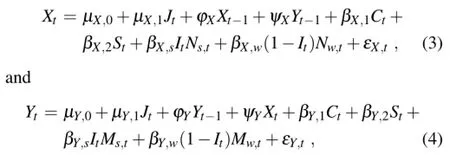
whereµ(X,0),µY,0,µX,1,µY,1,ϕX,ϕY,ψX,ψY,βX,1,βX,2,βY,1, βY,2,βX,s,βX,w,βY,sandβY,ware model coefficients.Ns,tand Nw,t(Ms,tand Mw,t)are the LOESS-smoothed summer and winter seasonal mean minimum(maximum)temperatures. Here,the two error terms,εX,tandεY,t,besides being normally distributed with zero means,have no autocorrelation or cross correlation.

Note that the seasonal indicators in Eqs.(1-4)allow for differentrelationshipswith theaggregatedcovariatesdepending on the season.The degree of LOESS smoothing is determined by the criterion based on minimizing the overdispersion phenomenon,through trial and error ranging from the case of no smoothing to as smooth as possible.Kim et al. (2012)considered the same degree of smoothness(i.e.,0.4) in all GLM models at the two locations.

Kim et al.(2012)illustrated that the proposed model virtually eliminates the overdispersion phenomenon in nearly all cases in reproducing variances of annual,as well as summer and winter,total precipitation(mm)and mean minimum and maximumtemperatures(◦C)attwolocationsintheArgentine Pampas,Pergamino and Pilar.Both locations have a marked wet season in the Southern Hemisphere summer.They also reported that the results(not shown)were not very sensitive to the precise value of the parameter governing the degree of smoothing in LOESS(e.g.,the overdispersion in the summer total precipitation at Pergamino was still virtually eliminated if the degree of smoothing was 0.5 instead of 0.4).It was noted that the introduction of the temporal trend in the temperature models was insufficient to correct the overdispersion,and the original model came close to reproducing the precipitation variability in winter.

In the application to downscaling seasonal forecasts(section 3),daily weather statistics,such as the total number of dry days and the median daily precipitation intensity within a season,are considered.It was verified that the GLM weather generator with aggregated covariates simulates the climatological distribution of these statistics reasonably well(results not shown).Furthermore,Kim et al.(2012)already extensivelyvalidatedtheproposedGLMweathergeneratorapplied to Pergamino and Pilar.

3.Downscaling seasonal forecasts

The IRI seasonal forecast product has been issued since October1997(Barnstonetal.,2010).Atpresent,theforecasts of seasonal total precipitation and mean temperature have at least a 0.5-month lead time(e.g.,the forecasts for the October through December season are released in mid-September). Seasonal forecasts with longer lead times of up to 3.5 months are also produced(e.g.,forecasts for the January through March season are also issued in mid-September).These IRI forecasts are probabilistic in nature,in that they are provided as a percentage likelihood in an A:N:B format,where“A”denotes the percentage chance of above-normal seasonal total rainfall,“N”denotes the percentage chance of near-normal rainfall,and“B”denotes the percentage chance of belownormal rainfall-and the three categories are typically based on the terciles.For example,a forecast of A:N:B=40:35: 25 for an area means that there is a 40%chance of seasonal total rainfall being above normal,a 35%chance of rainfall being near normal,and a 25%chance of below-normal precipitation.Forecasts of seasonal mean temperature are issued in the same format.

Barnston et al.(2010)thoroughly evaluated the skill of the IRI seasonal forecasts.Any such skill is necessarily limited,with the forecast probabilities frequently coinciding with climatology[i.e.,(1/3,1/3,1/3)]and only rarely being higher than 2/3 for a given category.Seasonal precipitation probability forecasts are reliable(i.e.,well-calibrated in the sense that they can be taken at face value),with the reliability of seasonal temperature forecasts suffering from a failure to correctly incorporate global warming trends.The forecast skill tends to match the strength of the ENSO signal,both in terms of geographic location and time of year.So,not surprisingly,there is some real,if small,skill for both precipitation and temperature during the Southern Hemisphere summer half of the year(October through March)in the ArgentinePampas[formoreinformationabouttheENSOsignal in the Argentine Pampas,see Furrer and Katz(2007)].This contribution of the ENSO phenomenon to the IRI forecasts is another reason for not including ENSO as a covariate in the GLM weather generator.

The IRI forecasts apply to a particular grid box,rather than a single location.As already mentioned,our approach is designed to deal with temporal,not spatial,downscaling.So, the IRI forecasts will be treated as if they apply to individual points.Because Pergamino and Pilar are closely situated, relative to the size of the grid boxes or the typical size of the contiguous area for which a deviation from climatology is predicted,the same IRI forecast probabilities always apply to both locations.Nevertheless,the downscaled daily weather statistics will differ both because of different downscaling relationships and because of different climatology(i.e.,as reflected in the coefficients in the GLM weather generators). Finally,the climate statistics used as covariates in the GLM were aggregated over six months,not three months as in the IRI seasonal forecasts.Rather than attempting to combine the IRI forecasts for two consecutive three-month periods(which are not always available for the second three months), we adopt the pragmatic approach of using the IRI forecasts for the first three months and only the climatology for the second three months.Stochastic weather generators based on the K-nearest neighbor resampling approach(Rajagopalan and Lall,1999;Beersma and Adri Buishand,2003;Apipattanavis et al.,2007)have been modified(Briggs and Wilks, 1996;Yates et al.,2003)to provide weather scenarios consistent with the seasonal probabilistic forecasts.We use this modification,first proposed by Yates et al.(2003)and used in Apipattanavis et al.(2007),in the current research.To the best of our knowledge,this is the first application of its kind to a GLM-based,or any other parametric,weather generator.

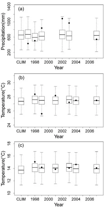
Fig.1.Downscaling of IRI forecasts for October to December 1997-2007,showing boxplots of the corresponding forecast distributions of summer(October to March)total precipitation (a),mean maximum temperature(b)and mean minimum temperature(c),along with the climatology(CLIM)and observed values(denoted by circles)for Pergamino.Boxplots are not shown for years in which the forecast coincides with the climatology.

The methodology proceeds as follows:(1)Historical years are classified into three categories-wet,normal and dry,based on the terciles of the smoothed historical summer(October-March)season precipitation(i.e.,consistent with the covariates used in the GLM weather generator).(2) The historical years are resampled with replacement based on the seasonal probabilistic forecast as the weight metric. Following the previous example of a 40:35:25 forecast, we would select years from the wet category with a 0.40 probability,normal years with a 0.35 probability,and dry years with a 0.25 probability.(3)The smoothed seasonal (October-March and April-September)precipitation values of the resampled years are used in the GLM weather generator as covariates to generate a rich variety of daily weather sequences at the point scale.An analogous approach is employed for the simulation of minimum and maximum temperature based on the seasonal forecast of mean temperature. The seasonal forecasts are available only for the mean temperatureandweassumethatitreflectstheminimumandmaximum temperatures as well.The resampling,step(2),is performed on the probabilistic forecast of the three-month seasonal mean temperature-and the corresponding smoothed seasonal(October-March and April-September)maximum and minimum temperatures are used in their respective GLM models as covariates.

Probability distributions of a suite of weather statistics (mentioned earlier)that are of importance in agricultural decision making will be computed,and compared with the corresponding climatological distribution to quantify the shift in theprobabilitiesandconsequentlytheriskestimates.Thisapproach has been demonstrated successfully in a resamplingbased weather generator(Apipattanavis et al.,2007)and has been applied to seasonal crop yield forecasts,quantifying delays in highway constructions,and in streamflow forecasts (Apipattanavis,2008;Apipattanavis et al.,2010a,2010b).

TodemonstratestatisticaldownscalingbasedontheGLM weather generator,we make use of the IRI seasonal forecasts issued in mid to late September for October through December in the years 1997 to 2007.For both total precipitationandmeantemperature,theforecastprobabilitiesdeviated from the climatology for only six of the 11 years.Figure 1 shows boxplots of the downscaled forecast probability distributions of summer(i.e.,October through March)total precipitation,maximum temperature,and minimum temperature at Pergamino.For comparative purposes,the corresponding boxplots for the climatological distributions are included as well,alongwiththeobservedseasonalstatisticsforeachforecast year(indicated by circles on the boxplots).

For total precipitation,the IRI seasonal forecasts with the greatest deviations from the climatology were for 1997,with a probability of 0.55 for the above-normal category,and for 1998,with a probability of 0.60 for the below-normal category.The consistent shift in the downscaled forecast boxplots toward wetter than normal conditions in 1997(drier in 1998)is evident in the figures,with the observed total precipitation being below normal for both years at Pergamino,but near normal for both years at Pilar.For mean temperature, the IRI seasonal forecasts with the greatest deviations from the climatology were for 1998 and 2003,with a probability of 0.50 for the above-normal category.The consistent shift in the downscaled forecast boxplots toward warmer than normal conditions for both maximum and minimum temperature is evident in the figures.In 1998,the observed seasonal mean maximum temperature was above normal at Pergamino,but near normal at Pilar,with the observed seasonal mean minimum temperature being above normal at both Pergamino and Pilar.In 2003,the observed mean maximum temperature wasbelow normal at Pergamino and near normal at Pilar,with the observed seasonal mean minimum temperature being above normal at Pilar,but near normal at Pergamino.

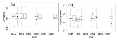
Fig.2.Downscaling of IRI forecasts for October to December 1997-2007,showing boxplots of the corresponding forecast distribution of the summer(October to March)mean number of dry days(a) and median daily precipitation intensity(b),along with the climatology(CLIM)and observed values (denoted by circles)for Pergamino.Boxplots are not shown for years in which the forecast coincides with the climatology.

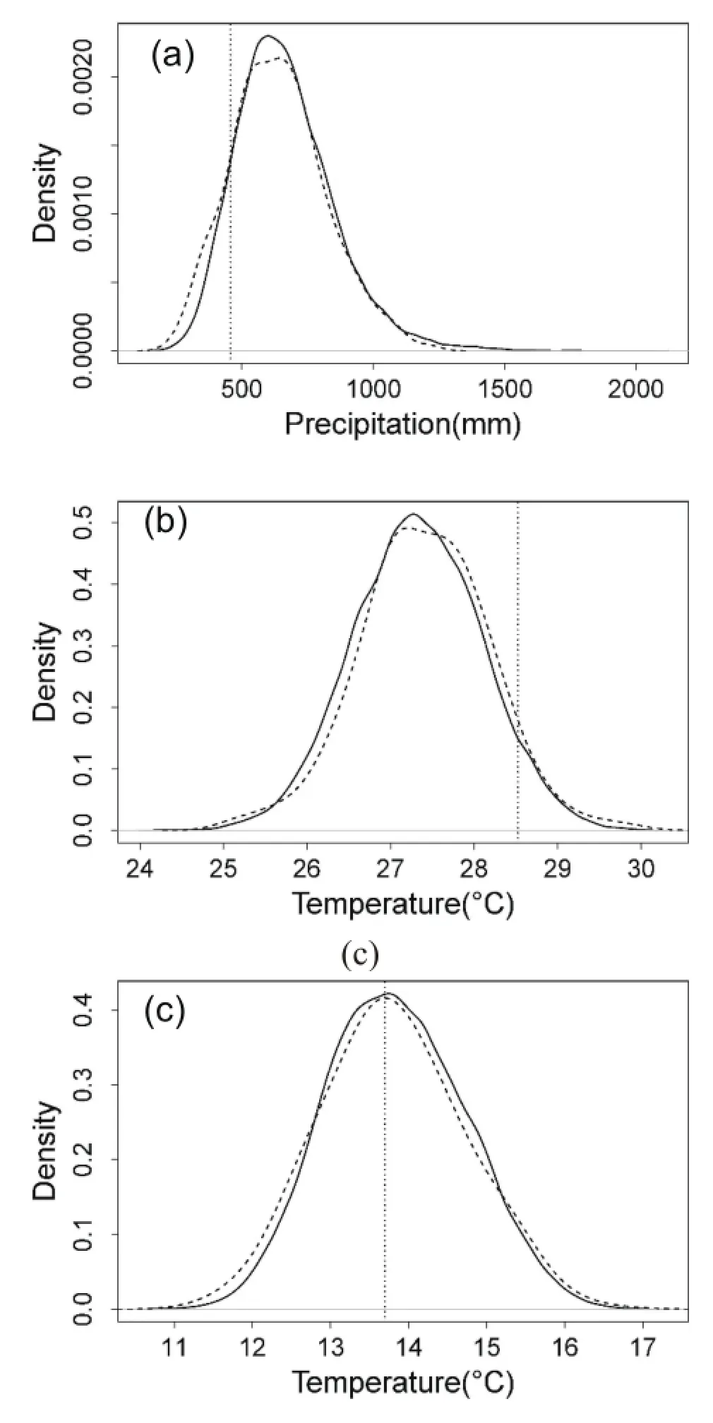
Fig.3.The PDF of summer precipitation(a),maximum temperature(b)and minimum temperature(c)from the simulation (dashed line),climatological PDF(solid line)and the observed value(vertical line)at Pergamino based on dry seasonal IRI forecasts(2004).

In an attempt to further downscale the IRI seasonal precipitation forecasts into more meaningful daily statistics,Fig. 2 shows boxplots of downscaled forecast probability distributions for the number of dry days and the median precipitation intensityatPergamino.Focusingagainon1997and1998,the years with the highest seasonal forecast probability of above-(or below-)normal total precipitation,the forecast boxplots of the number of dry days consistently shift toward less dry days in 1997(more dry days in 1998)and the boxplots of the median intensity consistently shift toward higher values in 1997(lower values in 1998).In 1997,the observed seasonal number of dry days was near normal at Pergamino and below normal atPilar,with the median intensity beingbelownormal at Pergamino but near normal at Pilar.In 1998,the observed seasonal number of dry days was near normal at Pergamino and below normal at Pilar,with the median intensity being below normal at both Pergamino and Pilar.

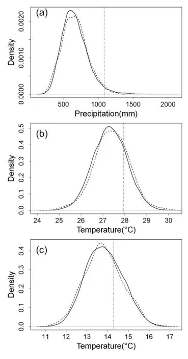
Fig.4.The PDF of summer precipitation(a),maximum temperature(b)and minimum temperature(c)from the simulation (dashed line),climatological PDF(solid line)and the observed value(vertical line)at Pergamino based on wet seasonal IRI forecasts(2000).

The performance of the downscaled seasonal forecasts shown in Fig.2 is evaluated using the ranked probability skill score(RPSS)(Wilks,2006,Chapter 7).The RPSS is calculated based on three categories at the tercile boundaries.RPSS=0 corresponds to no skill over the climatology, whereas RPSS=1 for perfect forecasts.In order to calculate the RPSS,the forecast probabilities of below normal,near normal,and above normal are first derived from the forecast probability density function(PDF)for each climate variable. At least limited skill is indicated for seasonal total precipitation,with RPSS=0.042 for Pergamino and RPSS=0.143 for Pilar.Because these forecasts apply to 6-month seasons, theirskillisnecessarilylessthanthatfortheoriginalIRIforecasts for the first half of the time period.

For seasonal mean minimum temperature the results are inconsistent,with RPSS=-0.015 for Pergamino but RPSS=0.073 for Pilar.Similarly,for seasonal mean maximum temperature,with RPSS=0.151 for Pergamino but RPSS=-0.118 for Pilar.Given that five out of 11 years had a climatological forecast,and in other years the climate forecast skill is modest at best,we do not expect a high overall RPSS value.This limited or lack of skill may be attributable in part to the original IRI forecasts being specified only in termsofmeantemperature,notminimumandmaximumtemperature,as mentioned earlier.

AclearshiftoftheforecastPDFofprecipitationtotheleft of the climatology,consistent with a dry forecast,can be seen at Pilar,but is not quite as apparent at Pergamino(Fig.3). However,the shift in the temperature PDFs to the right of the climatology,consistent with a warmer than normal temperature forecast probability,can be seen at both locations.The forecast PDFs of precipitation for the wet year of 2000 show similar consistent shifts relative to the climatology(Fig.4), but are somewhat subtler compared to the dry forecast case in Fig.1-and this can be attributed to the fact that the seasonal forecast for the dry year is closer to the climatology than that of the wet forecast.The shifts in the temperature PDFs are consistent with the IRI forecast representing nearnormal conditions.These shifts have significant implications for the tail probabilities,i.e.,the extremes and,consequently, crops yield impacts in agricultural applications.

We computed the PDFs of summer dry days(i.e.,total number of days with no rainfall)and hot days(i.e.,total number of days with maximum temperature above 35◦C)at the two locations for the dry year 2004(Fig.5).The shifts in the PDF of hot days at both locations relative to the climatology towards higher values,consistent with the shift in the PDF of mean maximum temperature(Fig.1),can be seen quite clearly,while the summer dry days exhibit weaker shifts.The corresponding results for the wet-year forecasts of 2000 are shown in Fig.6,with the most noticeable shift being toward a near normal number of hot days at Pilar.

4.Downscaling climate change scenarios

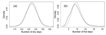
Fig.5.The PDF of the number of dry days(a)and hot days(b)from the simulation(dashed line)and climatological PDF(solid line)at Pergamino based on seasonal forecasts from IRI(2004).

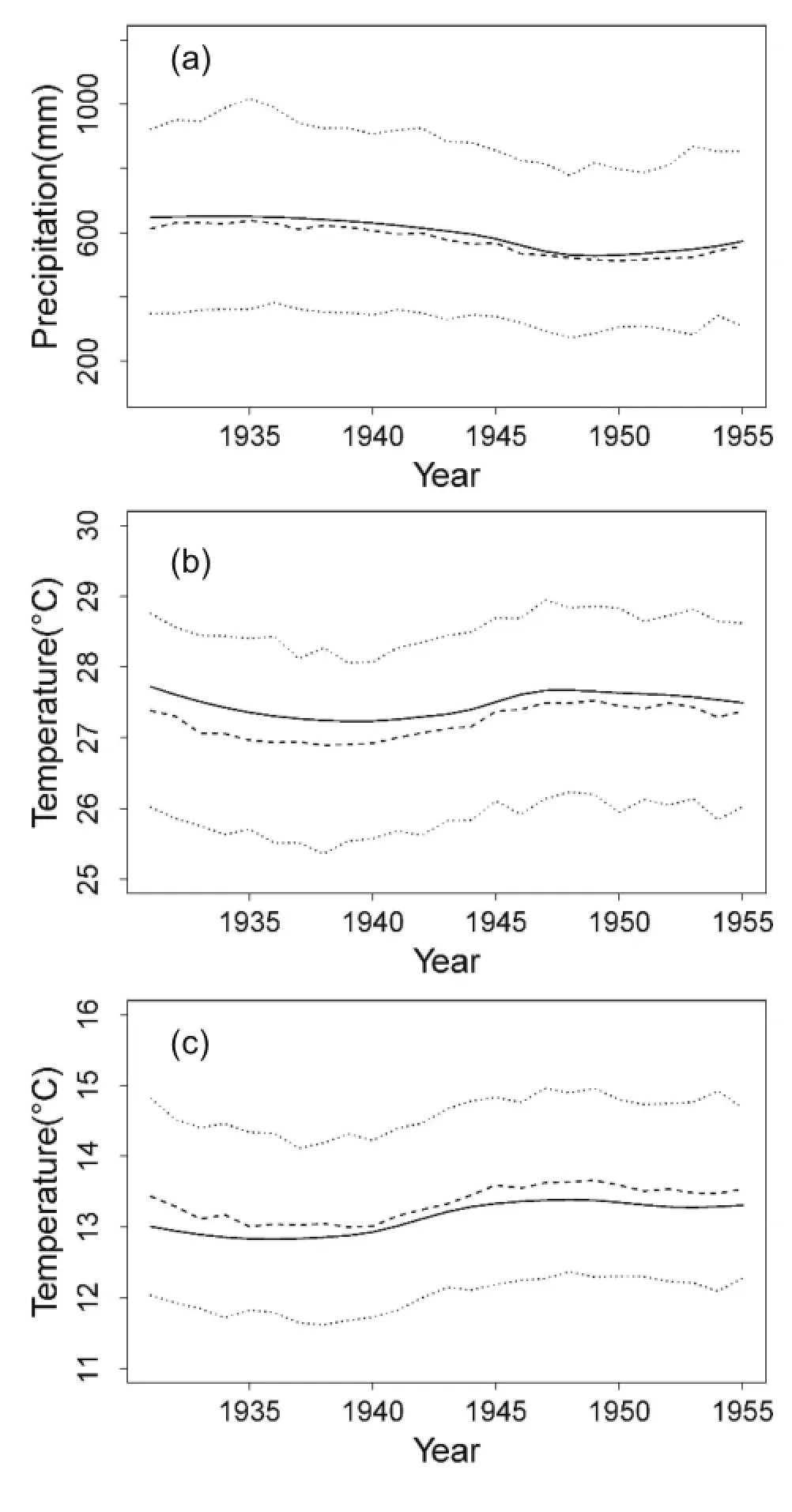
Fig.7.The simulated means(dashed line)and 95th projection band(dotted line)for summer seasonal total precipitation(a), mean maximum temperature(b)and mean minimum temperatures(c)during the 1931-55 epoch,along with the smoothed observed time series(solid line),for Pergamino.

Climate change projections for the 21st century are available at a monthly time scale and for a spatial scale given by the climate model grid-size(typically,hundreds of square kilometers)based on an ensemble of global climate change models(e.g.,the Fourth Assessment Report of the Intergovernmental Panel on Climate Change,IPCC AR4).For a point location,the time series of monthly precipitation and of temperature,consisting of the ensemble of climate change projections at the grid box containing the location,are considered for simplicity.Ensembles of weather sequences based on these projections can be generated by using the procedure described in the previous section-especially step(3).In particular,theseasonalprojectedvaluesofprecipitation,suitably smoothed,can be used as a covariate in the GLM weather generator described earlier to generate an ensemble of daily weather sequences consistent with the projections.This approach can also be used for downscaling shorter-term(e.g., decadal)projections.

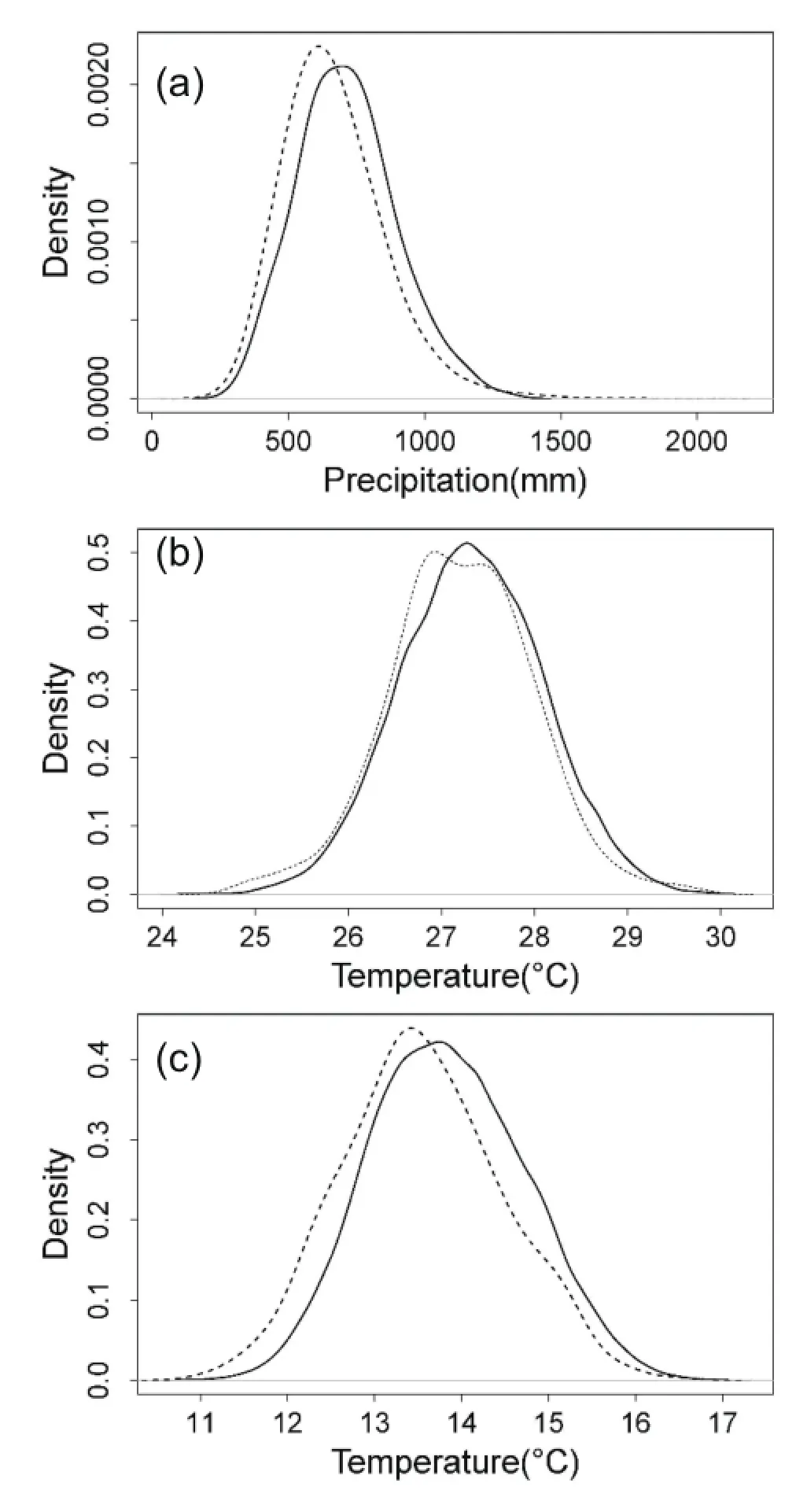
Fig.8.The PDF of the simulated projections(dashed line)of the summer total precipitation(a),mean maximum temperature (b)and mean minimum temperature(c)for the 1931-55 epoch, along with the model climatology(solid line),for Pergamino.

To demonstrate this approach,we selected an earlier dry epoch(1931-55)in the Argentine Pampas.The LOESS-smoothed seasonal precipitation and temperature for each year of these epochs were used a covariates to the GLM weather generator to produce daily weather sequences consistent with the decadal variability of these epochs.As before,probability distributions of a suite of weather statistics were computed and compared with the corresponding climatological distributions to check for epochal shifts.

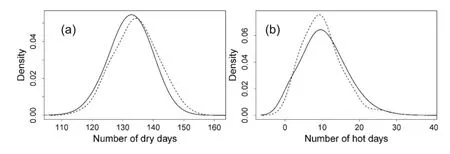
Fig.9.The PDF of simulated projections(dashed line)of the number of dry days(a)and hot days(b)for the 1931-55 epoch,along with the model climatology(solid line),for Pergamino.

The simulated summer seasonal precipitation,maximum and minimum temperature for the epoch,along with the projections at both locations,are shown in Fig.7.The 2.5th and 97.5th percentiles of the ensembles,the median and the smoothed time series projection during this epoch are shown in the figure.It can be seen that the ensembles track the projection very well at both locations,indicating that the methodologyisabletogenerateconsistentweathersequences with a rich variety.The PDFs from the simulations of the summer precipitation(Fig.8)both show clear shifts consistent with the drier epoch relative to the climatological PDF at both locations.Most noticeable shifts in temperature are towards lower minimum temperature at Pergamino.Shifts in the PDFs of summer dry days towards drier conditions are also clear at the two locations(Fig.9).

5.Conclusions

Using the incorporation of smoothed seasonally aggregated climate statistics into the GLM model as covariates,it has been demonstrated how the incorporation of such seasonally aggregated climate statistics facilitates statistical downscaling of seasonal climate forecasts.These results are encouraging in that the methodology provides a robust tool to generate weather sequences consistent with any seasonal climate forecast of potential use in resources planning and management.In the case of seasonal forecasts,the GLM weather generator makesit straightforwardto translate the uncertainty in the seasonal forecast product into that for the corresponding conditional daily weather statistics.

From a climate diagnostics perspective,it is somewhat uninformative to remove overdispersion through explicit use of seasonal aggregated climate statistics as covariates in the GLM weather generator.A more appealing approach could involve replacing these covariates with a hidden variable to reflect unobserved shifts in climate“regimes”on an interannual or longer(e.g.,decadal)time scale.Using a hidden Markov model(e.g.,MacDonald and Zucchini,1997)to represent this regime state would allow for long-term persistence,as well as having the advantage of being a fully probabilistic approach(i.e.,explicitly modeling the uncertainty about which climate regime is presently occurring).In addition,our approach can be applied in the spatiotemporal versions of GLM weather generators by using seasonal spatial average precipitation as the covariate(Verdin et al.,2015).

Acknowledgements.This research is supported by Korea Institute of Civil Engineering and Building Technology(Project name: 2015 Development of a micro raingauge using electromagnetic wave).

REFERENCES

Apipattanavis,S.,2008:Stochastic nonparametric methods for multi-site weather generation and flood frequency estimation:applications to construction delay,hydrology and agricultural modeling.PhD dissertation,University of Colorado, 199 pages.

Apipattanavis,S.,G.P.Podest´a,B.Rajagopalan,and R.W.Katz, 2007:A semiparametric multivariate and multisite weather generator.Water Resour.Res.,43,W11401,doi:10.1029/ 2006WR005 714.

Apipattanavis,S.,F.Bert,G.P.Podest´a,and B.Rajagopalan, 2010a:Linking weather generators and crop models for assessment of climate forecast outcomes.Agriculture and Forest Meteorology,150,166-174.

Apipattanavis,S.,K.Sabol,K.Molenaar,B.Rajagopalan,Y.Xi, B.Blackard,and S.Patil,2010b:Integrated framework for quantifying and predicting weather-related highway construction delays.Journal of Construction Engineering and Management,136,1160-1168.

Barnston,A.G.,S.H.Li,S.J.Mason,D.G.DeWitt,L.Goddard, and X.F.Gong,2010:Verification of the first 11 years of IRI's seasonal climate forecasts.Journal of Applied Meteorology and Climatology,49,493-520.

Beersma,J.J.,and T.Adri Buishand,2003:Multi-site simulation of daily precipitation and temperature conditional on the atmospheric circulation.Climate Research,25,121-134.

Benestad,R.E.,I.Hanssen-Bauer,and D.L.Chen,2008:Empirical Statistical Downscaling.World Scientific,228 pps.

Briggs,W.M.,and D.S.Wilks,1996:Extension of the Climate Prediction Center long-lead temperature and precipitation outlooks to general weather statistics.J.Climate,9, 3496-3504.

Buishand,T.A.,1978:Some remarks on the use of daily rainfall models.J.Hydrol.,36,295-308.

Caldwell,J.,B.Rajagopalan,and E.Danner,2014:Statistical modeling of daily water temperature attributes on the Sacramento River.Journal of Hydrologic Engineering,20, 04014065,doi:10.1061/(ASCE)HE.1943-5584.0001023.

Cleveland,W.S.,1979:Robust locally-weighted regression and smoothing scatterplots.Journal of the American Statistical Association,74,829-836.

Furrer,E.M.,and R.W.Katz,2007:Generalized linear modeling approach to stochastic weather generators.Climate Research, 34,129-144.

Giorgi,F.,and L.O.Mearns,1991:Approaches to the simulation of regional climate change:A review.Rev.Geophys.,29, 191-216.

Hansen,J.W.,and T.Mavromatis,2001:Correcting lowfrequency variability bias in stochastic weather generators. Agricultural and Forest Meteorology,109,297-310.

Hastie,T.J.,and R.J.Tibshirani,1990:Generalized Additive Models.Chapman and Hall.

Hostetler,S.W.,J.R.Alder,and A.M.Allan,2011:Dynamically downscaled climate simulations over North America:Methods,evaluation,and supporting documentation for users.U.S. Geological Survey Open-File Report 2011-1238,64 pp.

Katz,R.W.,and M.B.Parlange,1998:Overdispersion phenomenon in stochastic modeling of precipitation.J.Climate, 11,591-601.

Kim,Y.,R.W.Katz,B.Rajagopalanc,G.P.Podest´a,and E.M. Furrer,2012:Reduced overdispersion in stochastic weather generators using a generalized linear modeling approach.Climate Research,53,13-24.

MacDonald,I.L.,and W.Zucchini,1997:Hidden Markov and Other Models for Discrete-Valued Time Series.Chapman and Hall.

Mannig,B.,and Coauthors,2013:Dynamical downscaling of climate change in Central Asia.Global and Planetary Change, 110,26-39.

McCullagh,P.,and J.A.Nelder,1989:Generalized Linear Models.2nd ed.Chapman and Hall,206 pages.

Rajagopalan,B.,and V.Lall,1999:A k-nearest neighbor simulator for daily precipitation and other weather variables.Water Resour.Res.,35,3089-3101.

Richardson,C.W.,1981:Stochastic simulation of daily precipitation,temperature,and solar radiation.Water Resour.Res.,17, 182-190.

Stern,R.D.,and R.Coe,1984:A model fitting analysis of daily rainfall data.Journal of the Royal Statistical Society:Series A,147,1-34.

Verdin,A.,B.Rajagopalan,W.Kleiber,and R.W.Katz,2015: Coupled stochastic weather generation using spatial and generalized linear models.Stochastic Environmental Research and Risk Assessment,29,347-356.

Wilby,R.L.,and T.M.L.Wigley,1997:Downscaling general circulation model output:A review of methods and limitations. Progress in Physical Geography,21,530-548.

Wilby,R.L.,T.M.L.Wigley,D.Conway,P.D.Jones,B.C.Hewitson,J.Main,and D.S.Wilks,1998:Statistical downscaling of general circulation model output:A comparison of methods.Water Resour.Res.,34,2995-3008.

Wilby,R.L.,S.P.Charles,E.Zorita,B.Timbal,P.Whetton,and L.O.Mearns,2004:Guidelines for use of climate scenarios developed from statistical downscaling methods.Supporting material for Data Distribution Centre of Intergovernmental Panel on Climate Change.[Available online at http://www.ipcc-data.org/guidelines/dgm no2400 v1 09 2004.pdf].

Wilks,D.S.,1989:Conditioning stochastic daily precipitation models on total monthly precipitation.Water Resour.Res.,25, 1429-1439.

Wilks,D.S.,and R.L.Wilby,1999:The weather generator game: A review of stochastic weather models.Progress in Physical Geography,23,329-357.

Xu,Z.F.,and Z.L.Yang,2012:An improved dynamical downscaling method with GCM bias corrections and its validation with 30 years of climate simulations.J.Climate,25,6271-6286.

Yates,D.,S.Gangopadhyay,B.Rajagopalan,and K.Strzepek, 2003:A technique for generating regional climate scenarios using a nearest neighbor algorithm.Water Resour.Res.,39, 1199,doi:10.1029/2002WR001769.

Yoon,J.H.,L.Y.R.Leung,and J.Correia Jr.,2012:Comparison of dynamically and statistically downscaled seasonal climate forecasts for the cold season over the United States.J.Geophys.Res.,117,D21109,doi:10.1029/2012JD017650.

Kim,Y.,B.Rajagopalan,and G.Lee,2016:Temporal statistical downscaling of precipitation and temperature forecasts using a stochastic weather generator.Adv.Atmos.Sci.,33(2),175-183,

10.1007/s00376-015-5115-6.

8 May 2015;revised 20 July 2015;accepted 17 August 2015)

∗GyuWon LEE

Email:gyuwon@knu.ac.kr