Analysis of Hydrogen Permeation in Metals by Means of a New Anomalous Diffusion Model and Bayesian Inference

Marco A.A.Kappel,Diego C.Knupp,Roberto P.Domingosand Ivan N.Bastos

Analysis of Hydrogen Permeation in Metals by Means of a New Anomalous Diffusion Model and Bayesian Inference

Marco A.A.Kappel1,Diego C.Knupp1,Roberto P.Domingos1and Ivan N.Bastos1

This work is aimed at the direct and inverse analysis of hydrogen permeation in steels employing a novel anomalous diffusion model.For the inverse analysis,experimental data for hydrogen permeation in a 13%chromium martensitic stainless steel,available in the literature[Turnbull,Carroll and Ferriss(1989)],was employed within the Bayesian framework for inverse problems.The comparison between the predicted values and the available experimental data demonstrates the feasibility of the new model in adequately describing the physical phenomena occurring in this particular problem.

Anomalous diffusion,Hydrogen permeation,Bayesian inference,Inverse problems.

1 Introduction

Diffusion processes are quite frequently modeled by the classic Fick’s Law for conservation of species.Even though this model is able to describe very satisfactorily several processes,in some particular problems this approach fails to accurately describe the actual physical behavior[Bouchaud and Georges(1990)].This anomalous diffusion behavior is observed,for example,in the permeation of hydrogen in metals,due to temporary and permanent retention,or even sources of hydrogen atoms such as hydrade dissolution.Moreover,this process is strongly influenced by the presence of hydrogen traps such as grain boundaries,dislocations,carbides,and non-metallic particles[Turnbull,Carroll and Ferriss(1989)].In most works of the literature addressing this issue,the classical diffusion equation is adopted as the basic governing equation,but with the arbitrary introduction of sink and source terms to take into account these phenomena.For example,some works considered hydrogen diffusion with trapping[McNabb and Foster(1963)],rapid equilibrium between trapping and normal diffusion sites[Oriani(1970)],irreversible trapping[Iino(1982a);Iino(1982b)]or simultaneous reversible and irreversible trapping[Leblond and Dubois(1983a);Leblond and Dubois(1983b)],besides models that consider a varying degree of occupancy between reversible and irreversible trapping[Turnbull,Carroll and Ferriss(1989)].More general models,such as those based on fractional derivative equations[Metzler and Klafter(2000)],have become quite popular,with applications in several areas,such as diffusion in porous media,turbulence and complex materials(colloids,emulsions,biomaterials,etc.),among others,requiring the development of new numerical schemes for the solution of this class of problems[Chen and Sun(2009);Ray(2015);Wang,Liu,Chen,Liu and Liu(2015)].It should be highlighted that the understanding and adequate modeling of hydrogen diffusion in metals remains of paramount importance in engineering,since it significantly affects the mechanical behavior of steels[Tavares,Bastos,Pardal,Montenegro and da Silva(2015);Santos,Béreš,Bastos,Tavares,Abreu and da Silva(2015)].

Aiming at unifying all processes of diffusion with retention,Bevilacqua and coworkers derived a new analytical formulation for the simulation of the phenomena of anomalous diffusion[Bevilacqua,Galeão and Costa(2011a)],explicitly taking into account the retention effect in the dispersion process.In this new model,given by a fourth order differential equation,the blocking process is characterized by two additional parameters that arise naturally in the model,besides the classical diffusion coefficient.Some recent works investigated this new model from an inverse analysis perspective[Silva,Knupp,Bevilacqua,Galeão and Silva Neto(2014)],but to the best of our knowledge,a practical problem has not yet been analyzed through this approach.

Therefore,this work is aimed at the direct and inverse analysis,employing this new anomalous diffusion model,of the hydrogen diffusion in a 13%chromium martensitic stainless steel,with experimental data obtained in[Turnbull,Carroll and Ferriss(1989)]on successive hydrogen permeation tests.In order to estimate the parameters appearing in the proposed model,the Bayesian inference is employed for the inverse problem formulation[Kaipio and Sommersalo(2004)],with solution via Markov Chain Monte Carlo methods[Gamerman and Lopes(2006)].As further detailed in the remaining of the paper,the Bayesian framework is particularly adequate for this problem because of the existence of prior information regarding the lattice diffusion coefficient,as reviewed in[Kiuchi and McLellan(1983)].

2 Problem Formulation

Following the derivation described with details by Bevilacqua and co-workers,the anomalous diffusion model adopted in this work to describe the hydrogen con-centration in a given medium can be written as[Bevilacqua,Galeão and Costa(2011a)]:

where C is the hydrogen concentration,K2is the classical diffusion coefficient,which can be interpreted as the lattice(“true”)diffusion coefficient,for which a theoretical prior information is available in the literature(K2=7.2×10−5cm2/s at 23°C)[Kiuchi and McLellan(1983)],as also used in the analysis performed in[Turnbull,Carroll and Ferriss(1989)],β is the fraction of particles able to diffuse at each time step,K4is the complimentary coefficient related to the anomalous diffusion processes,and L is the membrane thickness.

The diffusion process modeled by Eq.1a is illustrated in Fig.1.At each time step,a fraction of the contents α pnof each nthcell is retained.The exceeding volume β pn,where β =(1−α),is divided between the neighboring cells,each one receiving 0.5β pnfor the case of symmetric distribution.If β =0 the model corresponds to the stationary solution,and for β=1 the classic formulation of pure diffusion is recovered.It should be highlighted that both additional parameters,β and K4,can,in principle,vary with time.However,in this work it is considered the simplest case,with constant coefficients,assuming all permanent hydrogen traps are already filled.

For the case of hydrogen permeation in membranes investigated in this work,the following boundary and initial conditions are considered:

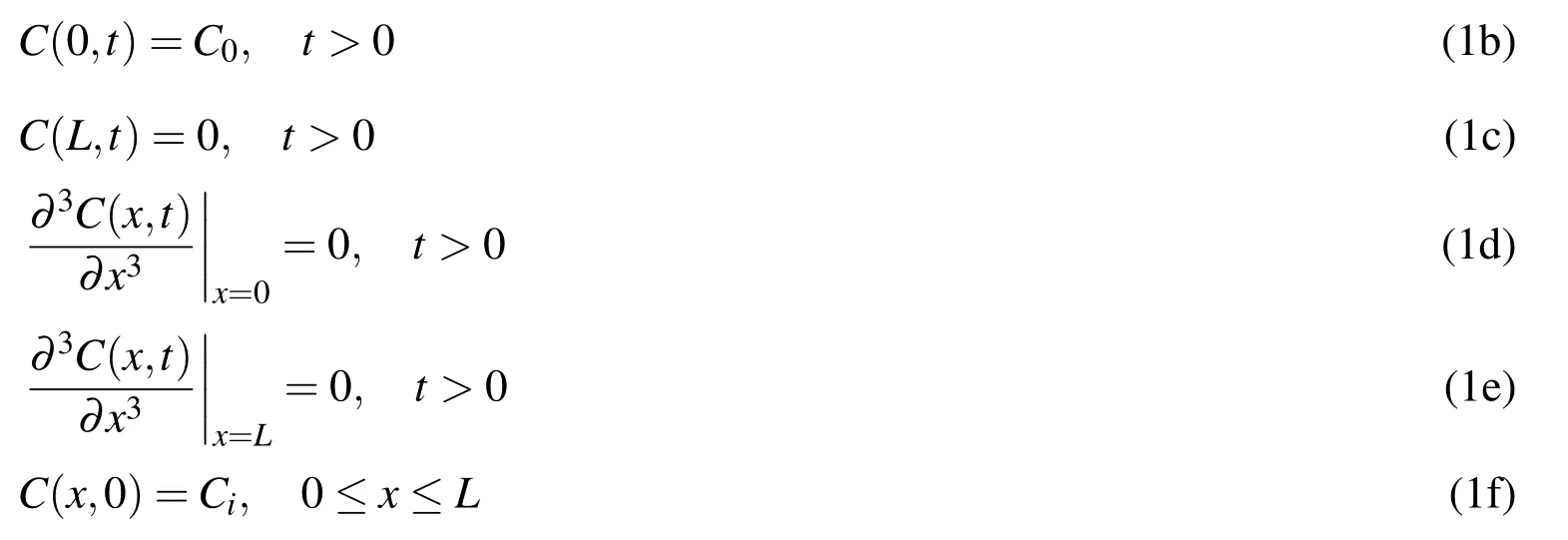
where C0is the hydrogen concentration prescribed at one side of the steel membrane,x=0,and Ciis the initial hydrogen concentration in the medium.It should be highlighted that the initial concentration actually refers to the hydrogen atoms able to diffuse,and therefore it is here considered zero even if in the second or third permeation,since in this work it is assumed that the hydrogen trapped in the previous permeations refer to permanent retention,not taken into account by this model.

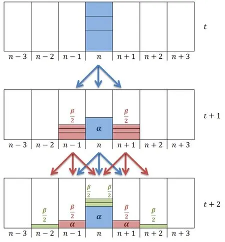
Figure 1:Schematic representation of the symmetrical distribution with retention α=(1−β)

The conditions Eq.1d and Eq.1e refer to null secondary flux at the boundaries[Bevilacqua,Galeão and Costa(2011b);Bevilacqua,Galeão and Costa(2011a)],i.e.it is assumed that there is no flux of retained hydrogen at the surfaces.

The problem given by Eq.1a–Eq.1f is solved with the NDSolve routine of the Wolfram Mathematica system[Wolfram(2005)],under automatic absolute and relative error control.This automatic solution path has been previous covalidated in previous works with the finite difference and finite element methods[Silva,Knupp,Bevilacqua,Galeão,Simas,Vasconcellos and Silva Neto(2013)].In order to calculate the hydrogen concentrations,information is needed on the values of the model parameters,K2,β and K4.As prior information is available for the lattice diffusion coefficient,K2[Kiuchi and McLellan(1983)],the critical objective is the estimation of β and K4from the available experimental data.In this work,the Bayesian approach for inverse problems is adopted as the basic framework,which allows for modeling the prior information regarding the parameter K2into the inverse problem formulation,as further discussed in the next section.

3 Inverse Analysis

Inverse problems are commonly classified as ill-posed problems,once the unique-ness of the solution is not guaranteed.Moreover,it is not stable with respect to the input data,i.e.,the experimental data,which contain the unavoidable measurement noise.Therefore,the solution of an inverse problem is not a trivial task,and many techniques have been proposed in the literature in order to overcome these difficulties.The most known and used approach is the maximum likelihood procedure.If the experimental errors are additive and can be modeled by a normal distribution with zero mean and constant standard deviation,and if the errors are not correlated,the maximum likelihood procedure leads to the very well known ordinary least squares objective function[Ozisik and Orlande(2000)].Even though this procedure can be very useful in several situations,the maximum likelihood approach does not allow for the incorporation of prior information,which eventually can be available for one or more parameters,such as the case of the lattice diffusion coefficient,K2,appearing in Eq.1a,which allows for modeling a theoretical prior information,as discussed in[Kiuchi and McLellan(1983)].In this scenario,the Bayesian approach for inverse problems[Kaipio and Sommersalo(2004)]is employed in this work.

The main purpose of the Bayesian approach is to calculate the posterior probability distribution for the parameters,from the prior knowledge of their distributions,aggregated with the available experimental data.The inverse problem is formulated as a problem of statistical inference and it is based on four basic principles[Kaipio and Sommersalo(2004)]:(i)All variables of the model are modeled as random variables;(ii)The randomness describes the degree of information;(iii)The degree of information is coded in probability distributions;(iv)The solution of the inverse problem is the posterior probability distribution.Thus,in the Bayesian approach all possible information is incorporated in the model,yielding a better uncertainty assessment of the estimated parameters.

Considering the prior information available on the model parametersZcan be modeled as a probability density πpr(Z),the Bayes theorem for inverse problems can be expressed as[Kaipio and Sommersalo(2004)]:

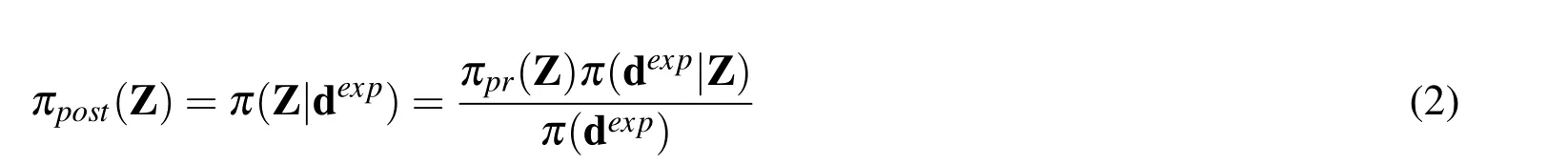
where πpost(Z)is the posterior probability density,πpr(Z)is the prior information on the unknown parameters,modeled as a probability distribution,π(dexp)is the marginal density and plays the role of a normalizing constant,and π(dexp|Z)is the likelihood function.Considering the measurement errors related to the datadexpare additive,uncorrelated,and have normal distribution,the probability density for the occurrence of the measurementsdexpwith the given parameters valuesZcan be expressed as[Beck and Arnold(1977)]:

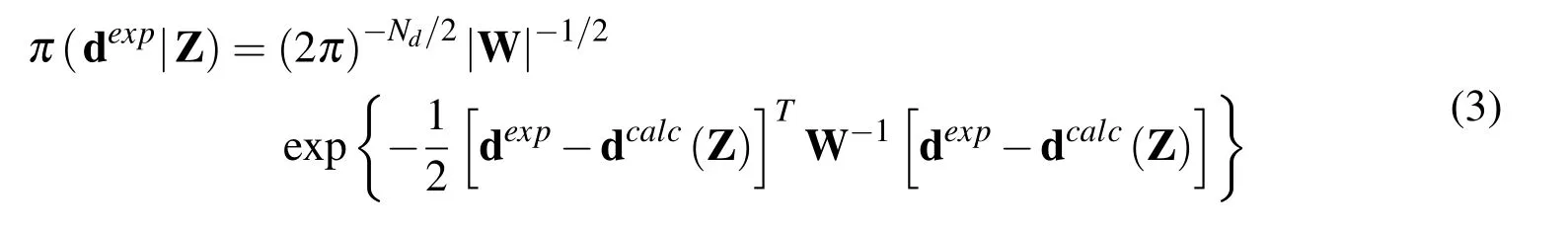
whereWis the covariance matrix,related to the experimental datadexp,anddcalcare the calculated data,obtained from the mathematical model solution employing the parametersZ.

This methodology produces a distribution which might be explored in different ways,using different methods.One of the most common approaches to obtain the estimates is through the maximum a posteriori(MAP)estimator[Knupp,Silva,Bevilacqua,Galeão and Silva Neto(2014)],but one way of directly exploring the posterior probability distribution is through random sampling methods,such as the Markov Chain Monte Carlo(MCMC)techniques[Kaipio and Sommersalo(2004);Gamerman and Lopes(2006)].

The present work uses the Metropolis-Hastings algorithm[Kaipio and Sommersalo(2004);Gamerman and Lopes(2006)]to implement the MCMC method.First,a candidate-generating density function q(Zt,Z∗)must be implemented.This function gives the probability of choosing a candidateZ∗from the current state of the chain,Zt.The following algorithm describes the procedure used in this work:

Step 1:Sample a candidateZ∗from the current stateZt,employing the candidategenerating density q(Zt,Z∗)

Step 2:Calculate

Step 3:IfU(0,1)＜α,then

else

where U(0,1)is a random number from a uniform distribution between 0 and 1.

Step 4:Return toStep 1in order to generate the chain?Z1,Z2,...,ZNMCMC?.It should be mentioned that the first states of this chain must be discarded until the convergence of the chain is reached.These ignored samples are called the burn-in period,whose length will be denoted by Nburn-in.

In the present work we have used a random walk process in order to generate the candidates,so thatZ∗=Zt+η,where η follows the distribution q,which was defined as a normal density in this work.In this case q is symmetric and q(Z∗,Zt)=q(Zt,Z∗),so Step 2 is simplified and Eq.4 may be rewritten as:

4 Application

The experimental data used in the present work were directly obtained from the permeation measurements performed in[Turnbull,Carroll and Ferriss(1989)],in a 13%Cr martensitic stainless steel(AISI 410)commonly used for oil production tubing.The steel was quenched and double-tempered as shown in Table 1.

Table 1:Chemical composition and heat treatment of AISI 410 stainless steel(mass%)[Turnbull,Carroll and Ferriss(1989)]

The permeation tests were performed using a Devanathan-Stachurski type cell[Turnbull,de Santa Maria and Thomas(1989);Devanathan and Stachurski(1962)],in which hydrogen is imposed at one side of the permeation membrane during cathodic polarization,whereas the other side of the membrane is kept at a given anodic potential.The measured current in this cell gives the instantaneous rate of hydrogen permeation through the membrane.The dimensionless current density J/J∞,as a function of the dimensionless time τ,is shown in Fig.2 for the third permeation experiment performed in[Turnbull,Carroll and Ferriss(1989)],where the steady state current J∞is calculated as:

and the dimensionless time is given by:

where C0=1.3×1017atom/cm3is the hydrogen concentration at x=0,and L=50 mm is the steel membrane thickness of the sample employed in the mentioned experiment[Turnbull,Carroll and Ferriss(1989)].

Regarding the model predictions,once the hydrogen concentration as function of position and time is calculated,C(x,t),as the solution of Eq.1a–Eq.1f,the current density,J,can be readily evaluated as:

where F is the Faraday constant.

The lattice diffusion,calculated with the classic Fick’s law(β =1 in Eq.1a),employing the lattice diffusion coefficient value,as obtained in[Kiuchi and McLellan(1983)],is also plotted in Fig.2,clearly demonstrating that the classical model is not able to describe the real physical dispersion phenomena occurring in this application.

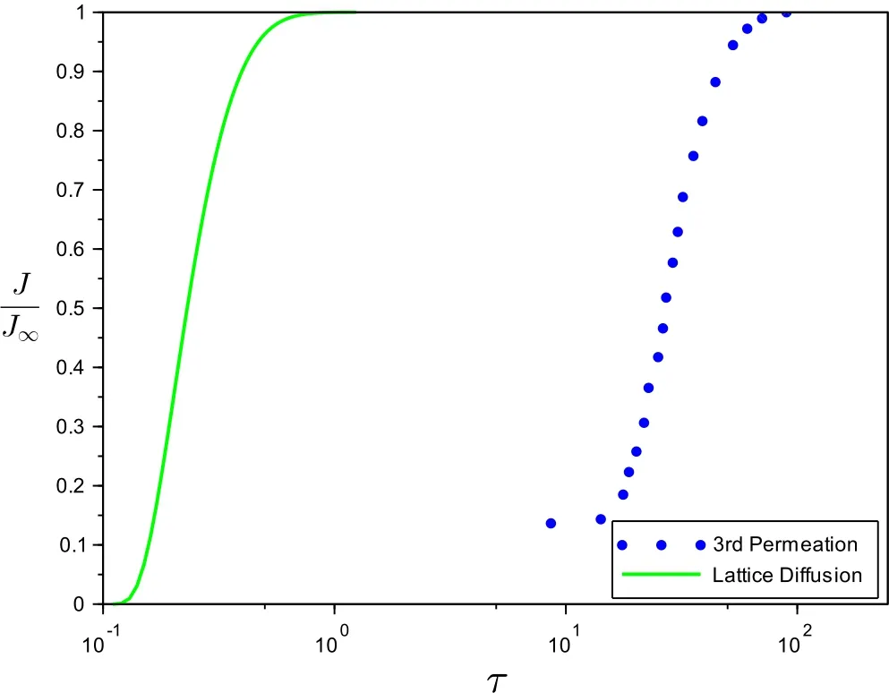
Figure 2:Dimensionless current transients during permeation for AISI 410 stainless steel in acidified NaCl at 23°C.Experimental data from[Turnbull,Carroll and Ferriss(1989)]

5 Results and Discussion

In order to solve the inverse problem for the estimation of the model parameters appearing in Eq.1a with the MCMC method,described in Section 3,the currentdensity measurements for the third permeation test,presented in Fig.2,are employed as the experimental data,dexp.These measurements were directly extracted from[Turnbull,Carroll and Ferriss(1989)],and in the absence of further information regarding the characterization of the experimental error,the measurement fluctuations were considered to follow a normal distribution with zero mean,no correlation,and constant standard deviation.Hence,the covariance matrixW,in the likelihood function,Eq.3,is constituted by a diagonal matrix with the experimental constant variance,σ2.In this case,considering the precision reported in[Turnbull,Carroll and Ferriss(1989)],the experimental standard deviation was considered as σ=0.01.For the calculated values,dcalc(Z)in Eq.3,onceC(x,t)is calculated,as the solution of Eq.1a–Eq.1f employing the valuesZfor the model parameters,Eq.10 is employed to calculate the current density,which is in fact the desired quantity to compare with the experimental data.

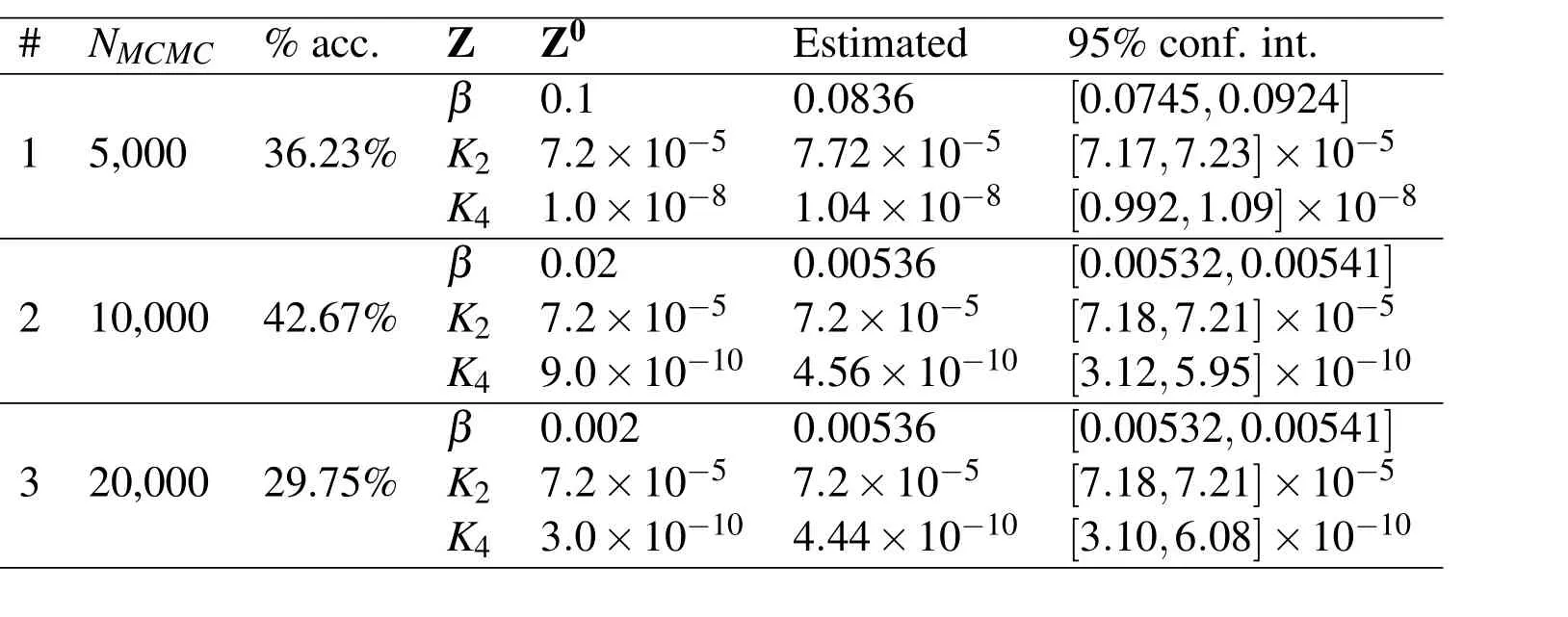
Table 2:Estimated parameters with the Bayesian inference via MCMC([K2]≡cm2/s,[K4]≡cm4/s)

For the prior information modeling,πpr(Z)in Eq.2,it was considered for the parameter K2a normal distribution with mean µK2=7.2×10−5cm2/s[Kiuchi and McLellan(1983);Turnbull,Carroll and Ferriss(1989)].Since no uncertainty assessment was reported for this value,it was here assumed a quite reliable prior information,with σK2=10−7cm2/s(＜ 0.15%ofµK2).For the parameters β and K4non-informative priors(uniform distributions)were employed.Tab.2 summarizes three runs of the MCMC algorithm,considering different initial states in the Markov Chain for the parameters β and K4,for which prior information are not available.For the parameter K2the available prior information,µK2,was considered as the initial state in all cases.The candidate-generating density q was chosen as a normal distribution with mean given by the current state,and the standard deviation empirically adjusted as 2%of the initial state,10−7,and 10%of the initial state for β,K2and K4,respectively,in order to roughly achieve a 30%acceptance ratio.From the first run,constructed with a total of 5,000 states with the first 1,000 states discarded as the burn-in,to the second,constructed with a total of 10,000 states with the first 2,000 states discarded as the burn-in,it is clear,from the divergent estimated confidence intervals,that the chains were still not converged for NMCMC=5,000.On the other hand,comparing the second and third runs,constructed with 10,000 and 20,000 states,respectively(both with the first 2,000 s-tates discarded as the burn-in),employing different initial states,one can clearly observe that the chains are converged,with the estimated 95% confidence intervals being remarkably similar for all three parameters.

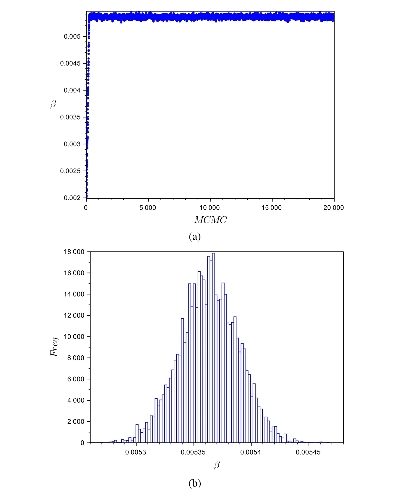
Figure 3:(a)Markov chain evolution and(b)inferred histogram of the posterior probability density function for the parameter β

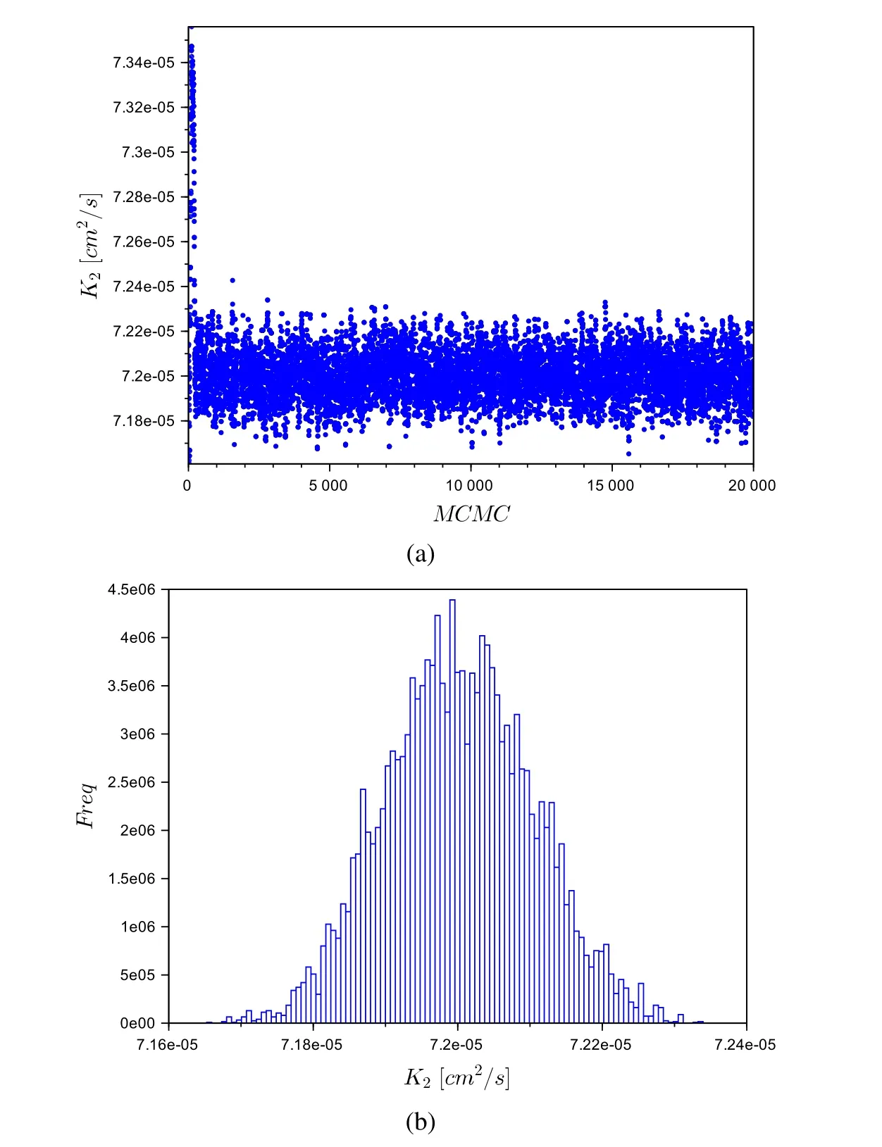
Figure 4:(a)Markov chain evolution and(b)inferred histogram of the posterior probability density function for the parameter K2

Fig.3 to Fig.5 depict the Markov chain evolution for the third run presented in Tab.2 as well as the inferred histogram of the posterior probability density function for all three parameters β,K2and K4,respectively.These results clearly demonstrate that the chains achieve the equilibrium distributions quite rapidly in the present case,clearly illustrating that the first 2,000 states,discarded as the burn-in,is more than enough to achieve the equilibrium of the chains.Moreover,from the histograms,one observes that the posterior probability density functions of all three parameters tend to normal distributions.

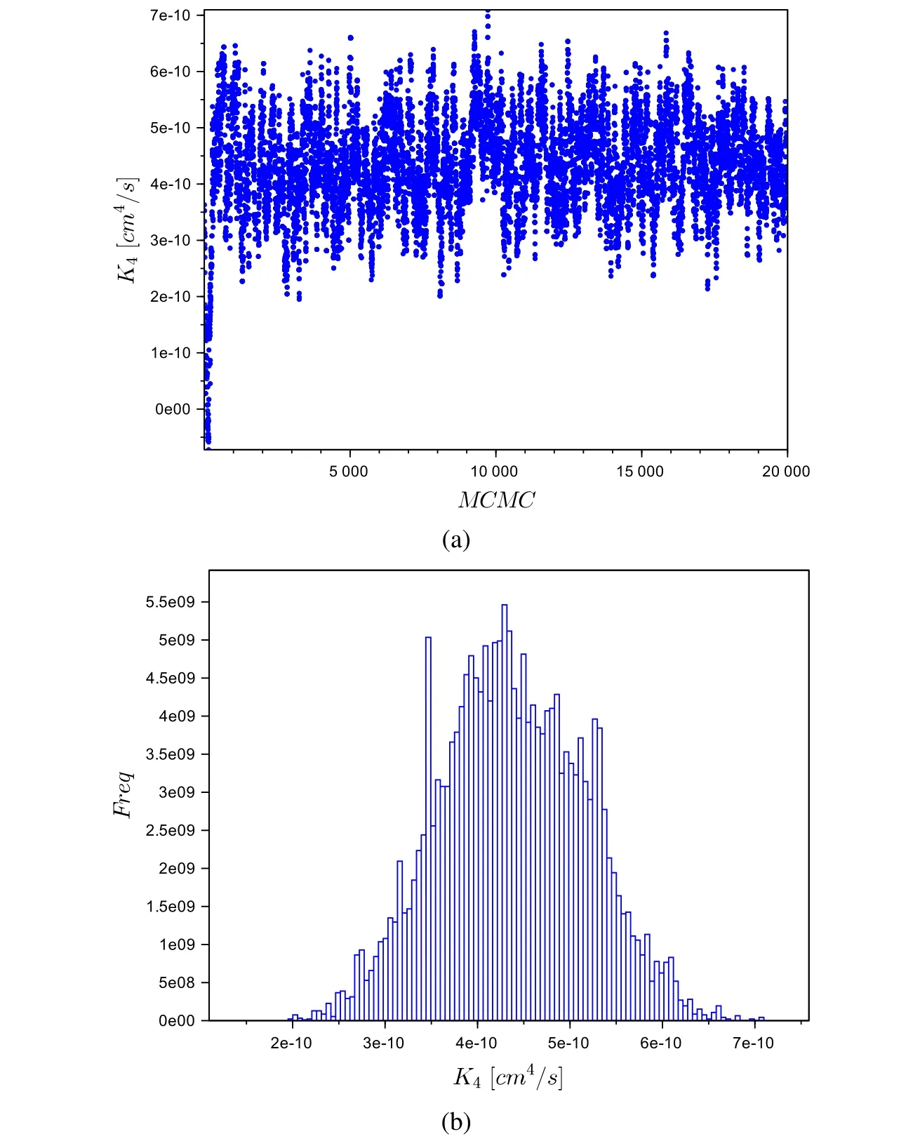
Figure 5:(a)Markov chain evolution and(b)inferred histogram of the posterior probability density function for the parameter K4

After con firming the good convergence behavior of the Markov chains constructed through the inverse problem solution,we now investigate the solution behavior of the anomalous diffusion model,Eq.1a to Eq.1f,regarding the hydrogen concentration distribution within the steel membrane,employing the estimated parameters.

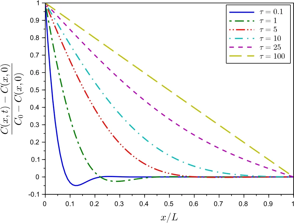
Figure 6:Calculated dimensionless hydrogen concentration in the stainless steel membrane for different instants(3rdpermeation test)

Fig.6 depicts the calculated dimensionless hydrogen concentration along the stainless steel plate,from x=0 to x=L,at different instants.It is interesting to notice that at the early stages,the predicted hydrogen concentration is below zero at some positions.As reported in the careful numerical study carried out by Bevilacqua and co-workers[Bevilacqua,Galeão and Costa(2011b)],this phenomenon is associated with a counter- flux process when the decaying speed of the concentration exceeds the one corresponding to the classical diffusion equation.This solution is physically compatible if there is a local stock able to supply particles.Indeed,it can be the case in the particular problem of hydrogen permeation in a medium with reversible traps,since during the third permeation here considered it is expected that a fraction of hydrogen atoms is trapped within the metal structure,being able to supply this flux.It should be recalled that the zero concentration level,here imposed as the initial condition,actually refers to hydrogen atoms not permanently trapped within the membrane.On the other hand,if a sufficient supply is not available,the model would be no longer valid and,physically,the concentration continuity would be broken,yielding instability in the diffusion process.This can be the case in the earlier permeations,and could explain,at least in part,the embrittlement caused by hydrogen diffusion in steels,since the permanent hydrogen-metal interaction can cause mechanical damage.

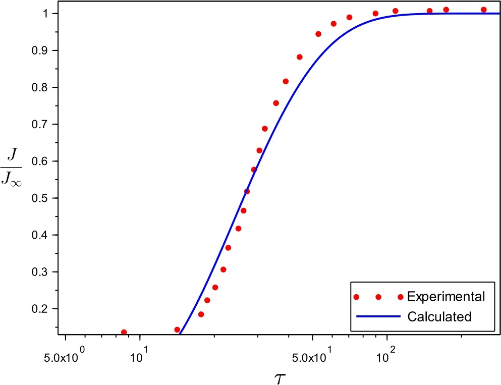
Figure 7:Calculated current density after the inverse problem solution and comparison against experimental data[Turnbull,Carroll and Ferriss(1989)]

Finally,the current density as calculated with Eq.10 with the predicted hydrogen concentration,C(x,t),is compared with the experimental measurements obtained in[Turnbull,Carroll and Ferriss(1989)].These results are depicted in Fig.7,illustrating an excellent adherence of the predicted values,as calculated from the anomalous diffusion model here employed,with the experimental data,demonstrating the feasibility of this model in accurately describing the diffusion process in hydrogen permeation.

6 Conclusions

The hydrogen permeation process within a medium has been investigated by means of a new anomalous diffusion model.In order to estimate the model parameters,the Bayesian framework for inverse problems was adopted,employing experimental data available in the specialized literature for a 13%chromium martensitic stainless steel[Turnbull,Carroll and Ferriss(1989)].The new model was demonstrated to accurately describe the real physical phenomena,bringing a new perspective to the analysis of hydrogen permeation in steels.A counter- flux behavior was predicted in the early stages of successive permeation,indicating that the concentration continuity may be broken in some circumstances,if the stock of hydrogen trapped in the medium is not enough to supply this demand,yielding instability of the diffusion process.This phenomenon is not predicted in diffusion models that only consider the Fickian flux of hydrogen,even in successive permeations.

Acknowledgement:The authors acknowledge the financial support provided by the Brazilian sponsoring agencies CNPq and FAPERJ.

Beck,J.V.;Arnold,K.J.(1977): Parameter Estimation in Engineering and Science.Wiley,New York.

Bevilacqua,L.;Galeão,A.C.N.R.;Costa,F.P.(2011a): A new analytical formulation of retention effects on particle diffusion processes. Annals of the Brazilian Academy of Sciences,vol.83,no.4,pp.1443–1464.

Bevilacqua,L.;Galeão,A.C.N.R.;Costa,F.P.(2011b):On the significance of higher order differential terms in diffusion processes.Journal of the Brazilian Society of Mechanical Sciences and Engineering,vol.33,no.2,pp.166–175.

Bouchaud,J.-P.;Georges,A.(1990): Anomalous diffusion in disorded media:Statistical mechanisms,models and physical applications.Physics Reports,vol.195,no.4-5,pp.127–293.

Chen,W.;Sun,H.(2009):Numerical solution of fractional derivative equations in mechanics:advances and problems.In ICCES:International Conference on Computational&Experimental Engineering and Sciences,volume 9,pp.215–218.

Devanathan,M.;Stachurski,Z.(1962): The adsorption and diffusion of electrolytic hydrogen in palladium.In Proceedings of the Royal Society of London A:Mathematical,Physical and Engineering Sciences,volume 270,pp.90–102.The Royal Society.

Gamerman,D.;Lopes,H.F.(2006): Markov Chain Monte Carlo:stochastic simulation for Bayesian inference.Chapman&Hall/CRC,2nd edition.

Iino,M.(1982a):Analysis of irreversible hydrogen trapping.Acta Metallurgica,vol.30,no.2,pp.377–383.

Iino,M.(1982b): A more generalized analysis of hydrogen trapping. Acta Metallurgica,vol.30,no.2,pp.367–375.

Kaipio,J.;Sommersalo,E.(2004): Statistical and Computational Inverse Problems.Springer-Verlag.

Kiuchi,K.;McLellan,R.(1983):The solubility and diffusivity of hydrogen in well-annealed and deformed iron.Acta Metallurgica,vol.31,no.7,pp.961–984.

Knupp,D.C.;Silva,L.G.;Bevilacqua,L.;Galeão,A.C.N.R.;Silva Neto,A.J.(2014): Uncertainty analysis in the solution of an inverse anomalous diffusion problem employing maximum likelihood and bayesian estimation.In Proceedings of 17th Scientific Convention on Engineering and Architecture,November 24-28,2014,Havana,Cuba.

Leblond,J.;Dubois,D.(1983a):A general mathematical description of hydrogen diffusion in steels-i.derivation of diffusion equations from Boltzmann-type transport equations.Acta Metallurgica,vol.31,no.10,pp.1459–1469.

Leblond,J.;Dubois,D.(1983b):A general mathematical description of hydrogen diffusion in steels-ii.numerical study of permeation and determination of trapping parameters.Acta metallurgica,vol.31,no.10,pp.1471–1478.

McNabb,A.;Foster,P.(1963):A new analysis of the diffusion of hydrogen in iron and ferritic steels.Transactions of the Metallurgical Society of AIME,vol.227,pp.618.

Metzler,R.;Klafter,J.(2000):The random walk’s guide to anomalous diffusion:a fractional dynamics approach.Physics Reports,vol.339,no.1,pp.1–77.

Oriani,R.A.(1970): The diffusion and trapping of hydrogen in steel. Acta Metallurgica,vol.18,no.1,pp.147–157.

Ozisik,M.N.;Orlande,H.R.B.(2000): Inverse Heat Transfer:Fundamentals and Applications.Taylor&Francis,New York.

Ray,S.S.(2015):A new coupled fractional reduced differential transform method for the numerical solution of fractional predator-prey system.CMES:Computer Modeling in Engineering&Sciences,vol.105,no.3,pp.231–249.

Santos,L.;Béreš,M.;Bastos,I.;Tavares,S.;Abreu,H.;da Silva,M.G.(2015):Hydrogen embrittlement of ultra high strength 300 grade maraging steel.Corrosion Science,vol.101,pp.12–18.

Silva,L.;Knupp,D.;Bevilacqua,L.;Galeão,A.;Simas,J.;Vasconcellos,J.;Silva Neto,A.(2013): Investigation of a new model for anomalous diffusion phenomena by means of an inverse analysis.In Proceedings of the 4th Inverse Problems,Design and Optimization Symposium-IPDO 2013,Albi,France.

Silva,L.G.;Knupp,D.C.;Bevilacqua,L.;Galeão,A.C.N.R.;Silva Neto,A.J.(2014): Inverse problem in anomalous diffusion with uncertainty propagation. Computer Assisted Methods in Engineering and Science,vol.21,pp.245–255.

Tavares,S.S.;Bastos,I.N.;Pardal,J.M.;Montenegro,T.R.;da Silva,M.(2015):Slow strain rate tensile test results of new multiphase 17%Cr stainless steel under hydrogen cathodic charging.International Journal of Hydrogen Energy,vol.40,no.47,pp.16992–16999.

Turnbull,A.;Carroll,M.;Ferriss,D.(1989): Analysis of hydrogen diffusion and trapping in a 13%chromium martensitic stainless steel.Acta Metallurgica,vol.37,no.7,pp.2039–2046.

Turnbull,A.;de Santa Maria,M.S.;Thomas,N.(1989): The effect of H2S concentration and pH on hydrogen permeation in AISI 410 stainless steel in 5%NaCl.Corrosion Science,vol.29,no.1,pp.89–104.

Wang,J.;Liu,L.;Chen,Y.;Liu,L.;Liu,D.(2015): Numerical study for a class of variable order fractional integral-differential equation in terms of Bernstein polynomials.CMES:Computer Modeling in Engineering&Sciences,vol.104,no.1,pp.69–85.

Wolfram,S.(2005):The Mathematica Book.Wolfram media,Cambridge.

1Instituto Politécnico,Universidade do Estado do Rio de Janeiro,Nova Friburgo,RJ,Brazil