RBFN stochastic coarse-grained simulation method:Part I-Dilute polymer solutions using Bead-Spring Chain models

H.Q.Nguyen,C.-D.Tranand T.Tran-Cong

RBFN stochastic coarse-grained simulation method:Part I-Dilute polymer solutions using Bead-Spring Chain models

H.Q.Nguyen1,C.-D.Tran1and T.Tran-Cong1

In this paper,dynamic behaviours of dilute polymer solutions of various bead-spring chain models in shear flow are studied using a coarse-grained method based on the Integrated Radial Basis Function Networks(IRBFNs)and stochastic technique.The velocity field governed by the macroscopic conservation equations is determined by the IRBFN-based method,whereas the evolution of configurations of polymer chains governed by the diffusion stochastic differential equations are captured by the Brownian Configuration Field(BCF)approach.The system of micro-macro equations is closed by the Kramers’expression,which allows for the determination of the polymer stresses in terms of BCF configurations.In this work,all nonlinear effects in a BSC model such as hydrodynamic interaction and excluded volume are considered.Since the simulation requires a considerable computational effort,parallel calculations are performed where possible.As an illustration of the method,the start-up planar Couette flow is examined,in which the evolution of viscometric functions such as shear stress,the first and the second normal stress differences is assessed with various BSC models.

Stochastic coarse-grained simulation,Brownian Configuration Fields,Integrated Radial basis function,nonlinear bead-spring chain models,hydrodynamic interaction,excluded volume.

1 Introduction

A polymer solution may be modelled as polymer chains suspended in a solvent.Polymer chains are represented by particles connected by some connector force laws.Several kinds of polymer chains have been used in polymer rheology as coarse-grained(CG)models of macromolecules,for example,the bead-rod chain,the bead-spring chain(BSC),and the worm-like chain.The BSC is a simple coarsegrained model of a polymer molecule,which can capture most of the important nonlinear rheological properties of polymer solution Bird,Curtiss,Armstrong,and Hassager(1987).Recently,the coarse-grained simulation methods have been developed and applied in several scientific and engineering areas because of their advantages in the simulation of soft matters,including complex viscoelastic fluids[Phan-Thien(2012)].Stochastic multiscale methods have also been introduced to model the constitutive relations and mechanical behaviour of concretes[Liu,Liu,Guan,He,and Yuan(2013);Liu,Liu,Yuan,He,and Mang(2014);Liu,Liu,Yuan,Mang,Zhang,Zhou,Yang,Du,Liang,and Yang(2014)].For polymeric fluids,the main idea of this approach is that the polymer-contributed stress is calculated averagely from a large ensemble of configurations of microstructures,which describe the real molecules existing in the polymer solutions.Meanwhile,the velocity field is determined by discretising the conservation equations.One scheme of this approach,namely the CONNFFESSIT[Laso and Ottinger(1993);Ottinger(1996)],is a stochastic macro-micro multiscale simulation method.Another scheme,known as Brownian Configuration Field(BCF)[Hulsen,Van Heel,and Van Den Brule(1997)],is based on the idea of an ensemble of configuration fields instead of using a collection of individual micro elements as in CONNFFESSIT.In an alternative approach,the combination of the Radial Basis Function Networks(RBFN)and the stochastic CG method has been suggested by Tran-Canh and Tran-Cong(2002).The method overcame the difficulties of complex meshing task by discretising the conservation equations on a set of collocation points using the high order RBFN approximation.As a result,the computed global stress tensor and velocity field with respect to time are very smooth.Furthermore,with a rather coarse set of collocation points,the method showed a stable and accurate solution for a range of problems,including planar Couette flow,Poiseuille flow,lid-driven cavity flow and 10:1 planar contraction flow[Tran-Canh and Tran-Cong(2002,2004);Tran,Phillips,and Tran-Cong(2009)].Recently,the method was further improved by introducing the integrated RBF(IRBF)based approximation instead of the differentiated/original RBF(DRBF)-based techniques to decrease the white noise in the stochastic simulation and increase the convergence rate of numerical solutions[Tran,An-Vo,Mai-Duy,and Tran-Cong(2011);Tran,Mai-Duy,Le-Cao,and Tran-Cong(2012)].In this paper,more complex BSC models are used to investigate the efficiency and adaptability of the IRBF-based stochastic CG method in the simulation of polymer solutions.

In the context of polymer kinetic theory,the simplest BSC model is the Rouse one,which represents the real polymer chain by a set of identical dumbbells,each of which consists of two beads linked by a Hookean spring[Rouse and Prince(1953)].

This model is very straightforward and is set up easily in Brownian dynamic simulations.However,the ability of the Rouse model to capture the properties of viscoelastic fluids or polymer solutions is very limited.There are only a few basic features of the dilute solution able to be predicted through the Rouse model,for example,the existence of a constant nonzero value of the first normal stress difference.However,other features,for example,the appearance of the nonzero second normal stress difference and the shear rate dependence of the viscometric functions cannot be predicted by the Rouse model[Bird,Curtiss,Armstrong,and Hassager(1987);Prakash(2001)].These limitations are due to(i)the existence of the Hookean law for the springs in the Rouse model,which can make the chain become infinitely extensible in shear/elongational flows and(ii)the neglect of intramolecular interactions of beads in a polymer chain such as the hydrodynamic interaction(HI)and the excluded volume(EV)effects.In order to improve the performance of the Rouse model,HI effect has been included in computational models in the equilibrium averaged form by Zimm(1956).As a result,the Zimm model has given better predictions of several properties of a polymer solution such as the diffusion coefficient and the relaxation time which are dependent on the molecular weight.Since both the Rouse and Zimm models are not successful in predicting the nonvanishing second normal stress difference as well as the dependence of viscometric functions on shear rate,the Finitely Extensible Nonlinear Elastic(FENE)spring-force law has been developed to resolve the limits of the Hookeanbased BSC models[Wedgewood,Ostrov,and Bird(1991);Herrchen and Ottinger(1997)].A number of significant advancements of the BSC model have been recently achieved to relevantly examine the effects of the intramolecular forces on the motion of molecular chains[Ottinger(1987b,1989);Magda,Larson,and Mackay(1988)].These improvements are very useful to predict the material properties of viscoelastic fluid flows and polymer solutions.By incorporating HI and EV into the simulations,the rheological characteristics including the existence of the second normal stress difference or the shear dependence of viscometric functions are accurately forecast[Ottinger(1989);Zylka(1991);Prakash(2001)].Thus,the obtained results from simulation are now able to be compared directly with those achieved from experiments.However,the considerable consumption of time and computer resources is a major hindrance in this simulation approach because the nonlinear intramolecular forces of each pair of beads in a chain needs to be calculated successively at each time step.This barrier can be overcome by introducing a parallel calculation into the simulation.Hence,the aim of this paper is to predict some rheological properties of polymer solutions in start-up shear flows,in which all nonlinear effects such as spring force laws,HI and EV are included using the IRBF-based stochastic CG method,taking advantage of parallel computation where possible.

The paper is organised as follows.Section 2 gives a short review of the governing equations of incompressible non-Newtonian fluid flows using the CG approach.In section 3,a stochastic CG simulation method is described in which the Brownian Configuration Field(BCF)technique for the computation of the polymer contributed stress is presented using different BSC models with/without nonlinear effects such as the HI and the EV.Specifically,the coupled macro-micro multiscale system for the BSC model is introduced together with its dimensionless forms in section 4.In section 5,the IRBF-based discretisation of governing macroscopic equations is introduced in details,followed by the explicit integration scheme for microscopic equations.A parallel computation for the microscopic simulation is also presented in this section.Numerical examples and obtained results are discussed in section 6.Finally,the paper is closed by a conclusion in section 7.

2 Stochastic coarse-grained method for dilute polymer solutions

Consider the flow of an isothermal and incompressible dilute polymer solution,a system of mass and momentum conservation equations is written as follows.

where u is the velocity field;τ is the total stress tensor given by

where τs=2ηsD and τpare stress components contributed by Newtonian solvent and polymer,respectively;ηsis the solvent viscosity;is the rate of strain tensor;pis the hydrostatic pressure and I is the unit tensor.

In a stochastic CG simulation method,the polymer-contributed stress(τp)can be calculated by directly solving the Fokker-Planck equation or the corresponding Stochastic differential equations(SDEs).The coupling of the conservation equations(Eqs.(1)and(2))and the equations expressing the evolution of grain configurations forms the basis for stochastic CG methods(Ottinger,1996;Phan-Thien,2012).In this work,the BCF-based stochastic CG method is used to describe the evolution of CG structures,and the non-Newtonian contribution to the stress is deduced from the evolution of coarse-grained configurations.This paper focuses on considering BSC models(Fig.1)with the effects of EV and HI.

Figure 1:Schema of a BSC model.The Latin subscripts(i,j,k,...)of a tensor/vector denote springs while the Greek ones(µ,ν,...)denote beads in a polymer chain;Qi=rµ+1-rµ.

3 The BCF-based stochastic CG method for BSC models

In the BCF approach,the general BSC model with all nonlinear effects,including HI and EV for the evolution of a connector vectorQi,is given as follows(Prabhakar and Prakash,2004).

where subscriptidenotes the index of connecting vectors(i=1，...，Ns);subscript µ indicates the index of beads(µ =1，...，Nb),µ =i;NsandNb=Ns+1 are the numbers of springs and beads,respectively in a polymer chain;u is the velocity field;ζ is the friction coefficient of the solvent;kBis the Boltzmann constant;Tis the absolute temperature of the solution and Wνis the Wiener process defined by an independent Gaussian variable with zero mean anddtvariance.ϒµνis the diffusion tensor and given by

where Ωµνand δµνare the hydrodynamic interaction tensor and the Kronecker delta,respectively.Ωµνis a function of vector rµν(rµν=rν-rµ)of the two beads µ and ν.It is worth noting that if µ and ν are two adjacent beads then rµνis the connector vector of spring(Q)between the two beads(Fig.1).Bµνis a second order tensor and determined by ϒµν=Bµν·BTµν.In the SDE(4),is the intramolecular interaction force,defined asand includes two components written as follows.

where φ is the potential energy;is the excluded volume force on bead ν by other beads in a chain andis the spring force by springs connected to bead ν and given by

whereHis the spring constant;is the connector vector of thekthspring(see Fig.1);Qkis the norm of Qkandb0is the square of dimensional maximum length/extension of thekthspring for the FENE dumbbell.

The system of multiscale governing equations Eqs.(1),(2)and(4)are closed by a connecting equation which determines the polymer stress contribution.For a coarse-grained model with intramolecular forces,the connecting equation known as Kramers’expression is given by[Bird,Curtiss,Armstrong,and Hassager(1987);Prakash(2002)]

wherenpis the number of polymer chains in a unit volume and the other parameters were defined as before.On the right-hand side of Eq.(9),the first term is the stress caused by the motion of beads in a polymer chain[Ottinger(1996)],the second term results from spring forces and the last term is produced by excluded volume interaction forces and given by[Prakash(2002)]

whereDνkare the entries of matrix Dνkof dimensionNb×Nsand defined asDνk=(k/Nb)-Θ(k-ν)where Θ(k-ν)is the Heaviside function.

3.1 Nonlinear properties of bead-spring chain model

3.1.1 Hydrodynamic interaction effect

HI is an indirect influence by the motion of beads through a solvent.Indeed,a bead moving in the solvent causes perturbations in the flow,which will influence the motions of remaining beads in the chain.The HI effect is incorporated into BSC models by introducing a hydrodynamic tensor Ωµνinto the equation of motion of beads.This tensor expresses the relationship between the force Fνexerted on bead ν and the velocity perturbation by other beadsµ’s in a polymer chain(µ =1，···，Nband µ /= ν)as follows.

A hydrodynamic tensor proposed by Rotne-Prager-Yamakawa(RPY)is given by[Rotne and Prager(1969);Yamakawa(1971)]

with

whereabis the bead radius defined by the Stokes law as ζ =6πηsab;rµνis the connecting vector between two beads µ and ν andrµνis the length/norm of vector rµν

An alternative formula of the hydrodynamic tensor Ωµνis established by Zimm(1956)as follows.

where all parameters were defined as before.

3.1.2 Excluded volume effect

The EV presence allows for an accurate prediction of the non-vanishing second normal stress difference and the shear rate dependence of viscometric functions of dilute polymer solutions.The EV effect can be incorporated into the simulation by introducing a forcein the convective term of Eq.(4).The force exerted on bead ν by the repulsive interactions from other beads µ’s in the chain is written by[Prakash(2001)]

whereEis the EV potential energy andEµνthe short-range function and given by[Prakash(2002)]

wherezis the solvent quality;Kis an arbitrary constant and χ is a known function ofbBSCand given spring force law.For example,χ=1 for the Hookean BSC model andfor the FENE BSC model[Sunthar and Prakash(2005)].

3.2 A coupled stochastic multiscale system

Collecting the conservation equations(1)-(2),the total stress formula Eq.(3),the stochastic BCF equation(4)and the Kramers’expression Eq.(9)yields a stochastic multiscale system as follows.

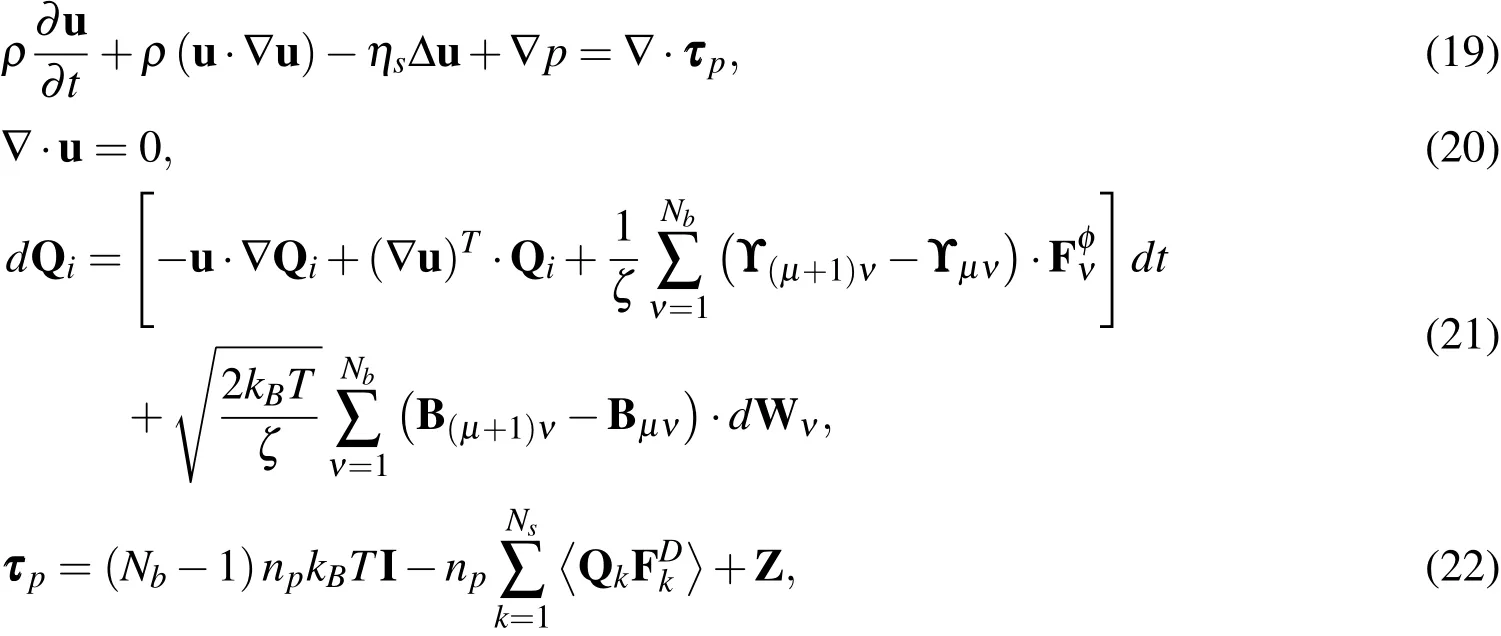
where all parameters were defined as before.

4 Non-dimensionalisation

Let U be a characteristic velocity;ηp=npkBTλHthe viscosity associated with the■polymers;λHandthe time scale and the characteristic length scale of the BSC polymer,respectively.Dimensionless variables are given as follows.

where ηo(ηo= ηs+ηp)is the total viscosity of the solution.

The dimensionless numbersRe,We,and ε are defined respectively as follows[Ottinger(1996);Laso and Ottinger(1993)].

The stochastic multiscale system Eqs.(19)-(22)is rewritten in the dimensionless form as follows.

wherebDis the square of dimensionless maximum extension of FENE dumbbell model and defined asbD=bBSCNs[Koppol,Sureshkumar,and Khomami(2007)].

The dimensionless form of Hookean and FENE spring forces(Eq.(8))and the EV interaction force Z(Eq.(10))are respectively rewritten as follows.

where the dimensionless form of the volume forceis given by

with

The RPY hydrodynamic tensor in Eq.(12)is expressed in the dimensionless form as follows[Prabhakar and Prakash(2004)].

with

Henceforth,all variables will be written in dimensionless form and the asterisk symbol will be removed for simplicity.

5 Numerical discretisation schemes

In this section,numerical schemes for the solution of the macro-micro system of differential equations are presented.Specifically,the deterministic PDEs(continuity and momentum equations)are approximated by a semi-implicit method based on IRBFNs while the evolution of the SDEs is determined using the Euler-Maruyama explicit scheme.

5.1 IRBF-based method for solution of the differential macroscopic governing equations

Consider the conservation equations(24)-(25).In order to solve this system,the problem domain is discretised using a set of nodal points,called the macro-scale grid.Here,instead of using the continuity equation(25),the incompressibility condition is enforced via the penalty method as follows[Laso,Picasso,and Ottinger(1997);Tran-Canh and Tran-Cong(2004)].

wherepeis a sufficiently large penalty parameter.Eqs.(24)-(25)and Eq.(35)yield the following equation

In this work,the 1D-IRBFN based semi-implicit scheme is employed to discretise the governing equation and presented in the next subsections.

5.1.1 Spatial discretisation

Consider an one-dimensional parabolic differential equation,at a time t,the highestorder derivative of the dependent variableu(x，t)(the second order in the case of this work)is decomposed as follows[Mai-Duy and Tran-Cong(2007)].

The corresponding first-order derivative and function itself are then determined through the direct integration as follows.

Collocating Eqs.(37),(39)and(40)at every grid pointyields the following set of algebraic equations

where

with

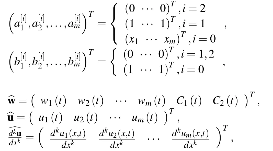
whereui=u(xi)withi=(1，2，...，m).

The presence of integration constants in the IRBFN based approximation yields beneficial mechanism for the incorporation of additional constraints such as nodal derivative values into the algebraic equation system.Thus,the algebraic equation system Eq.(43)can be reformulated as follows.

where D1and D2are known vectors of lengthm;andk2andk1are scalars determined byApplying Eq.(46)at every collocation point on the gridline yields

The values of the second and first order derivatives ofuin the IRBF form for a 2-D problem at all collocation points can be expressed similarly.More details can be found in Tran,An-Vo,Mai-Duy,and Tran-Cong(2011).

5.1.2 Time discretisation

A semi-implicit scheme(Crank-Nicolson)is employed to temporally discretise the momentum equation,which is solved for the velocity fielduat each time step where the polymer contributed stress τpis considered as a known variable from the microscopic procedure.Details will be presented in numerical examples in section 6.

5.2 Euler-Maruyama explicit scheme for solving microscopic SDEs

The evolution of the configuration of polymer chains in Eq.(26)using the Euler-Maruyama explicit scheme is given by[Ottinger(1996)]

where ∆tis the time step size;is the gradient of the known velocity field computed in the macroscopic procedure at the current time step;ϒ(µ+1)νand ϒµνare the diffusion tensors;is the intramolecular forces and Wνis the three-dimensional(3-D)Wiener process at bead ν.The diffusion tensors and intramolecular forces are calculated based on the configuration of all BS chains at time steptn.After a new configuration is obtained,the new polymer stress tensor is determined by Eq.(27)and its first order derivative is approximated using MQ-RBF as presented in section 5.1.1

5.3 Parallel computation

The stochastic macro-micro simulation requires considerable numerical computation.Furthermore,since the processing of tasks in the microscopic procedure dominates the throughput(Table 2),a parallel algorithm for the stochastic microscale simulation is incorporated into the present method to speed-up the computation.The stochastic tasks consist of:(i)solving SDEs and(ii)computing average stresses at collocation points.In general,these tasks are carried out independently for all configurations generated at each and every collocation point in the considered domain of a problem.

The parallel implementation of the algorithm is based on the message passing interface for parallel communication in Matlab environment.The implementation is carried out on the High Performance Computing system of the University of Southern Queensland whose details can be found inhttp://hpc.usq.edu.au.The parallelisation is established in regard to stochastic tasks at collocation points.In the framework of this paper,several results on the efficiency and speed-up are presented for the FENE-based BSC model,taking into account the HI and EV effects and discussed in section 6.4.

5.4 Algorithm of the present procedure

The present simulation method can now be described in a more detailed algorithm as follows and the implementation will be expressed in the illustrative examples.

(a)Generate a set of collocation points.Start with a given initial condition for the first iteration(velocity field,BSC configurations)together with the given boundary conditions of the problem.In the present work,the initial conditions are zero initial velocity field,and initial BSC configurations sampled from equilibrium Gaussian distribution.

(b)AssignNfbead-spring chains ofNssprings to each collocation point.All BSCs having the same index constitute a configuration field.Hence,there is an ensemble ofNfconfiguration fields.Since all the BSCs having the same index receive the same random number,there is a strong correlation between BSCs in a configuration field.

(c)Solving the macro PDEs for the velocity field using the 1D-IRBFN collocation method described in section 5.1;

(d)Solving the micro SDEs for the polymer configuration fields using the method presented in section 5.2.As mentioned in step(a),in order to ensure strong correlation within a configuration field,all the BSCs of the same index have the same random number;

(e)Determine the polymer contributed stress by taking the ensemble average of the polymer BSC configurations at each collocation pointxi,using Eq.(27).The tasks include the computation of the HI tensor(the RPY tensor in this work)and the EV interaction forces with regard to the hydrodynamic interaction and the excluded volume effects,respectively.Note:A parallel algorithm is installed within steps(d)and(e),see section 5.3 for details.

(f)With the stress field just obtained,approximate the gradient of stress field using the IRBFNs and then solve the macroscopic governing equation(36)for the new velocity field by the 1D-IRBFN method described in section 5.1;

(g)Terminate the simulation when either the desired time or convergence is reached.The latter is determined by a convergence measure(CM)for the velocity field,defined by wheredsis the number of dimensions;tola preset tolerance;uithei-component of the velocity at a collocation point;Nthe total number of collocation points andnthe iteration number.

(h)Return to step(d)for the next time step of the microscopic procedure until steady state or a given time is reached.

6 Numerical examples

The present method is employed to simulate the planar Couette flow described in Fig.2 using several BSC models.This problem with simpler polymer models was earlier studied by Laso and Ottinger(1993);Mochimaru(1983);Tran-Canh and Tran-Cong(2002,2004).Koppol,Sureshkumar,and Khomami(2007)studied the same problem using a finite element-based method.

Firstly,a creeping flow of viscoelastic fluid using FENE-BSC model which was considered in Koppol,Sureshkumar,and Khomami(2007)is simulated to assess the validity of the present method.The problem is then further investigated with the Rouse and Zimm models to study the HI effect on the rheological properties of the flow.Finally,the start-up problem is solved using general BSC models with fully nonlinear effects.

The problem is defined as follows.For timet＜0,the fluid is at rest.Att=0,the lower plate starts to move with a constant velocityV=1.No-slip condition is assumed at the walls.The fluid parameters of each considered BSC model mentioned above are presented in the next subsections.A set of collocation points is initialized uniformly along theydirection.Then the same number of BSC configurations is initiated randomly on each and every collocation point(see section 5.4,item a).

Figure 2:The start-up planar Couette flow problem.The collocation points and the velocity profile are only presented schematically.

The polymer stress field is calculated by Eq.(27)based on the initial BSC configurations.The obtained values by the microscopic procedure are located on the collocation points(i.e.micro-structural properties are transferred to a bulk property).These values at the grid points along with the boundary and initial conditions are used to start the simulation in the macroscopic procedure.The macroscopic governing equation is solved for the velocity field,and afterwards the transpose of velocity gradient(∇u)Tin the SDE(26)is defined by the IRBF-based approximation.All above calculations are repeated at each time step until the numerical convergence is satisfied.

6.1 Governing equations

From the characteristics of the start-up Couette flow of dilute polymer solution using the general BSC model,the system of stochastic multiscale equations(24)-(27)is developed as follows.

whereuis thex-component of the velocity;τpis the stresses of the flow including the shear stress τp，xy;Qi，x,Qi，yandQi，zare the components of connector vector Qiat locationy.is rowk(k=1，2，3)of matrixwith

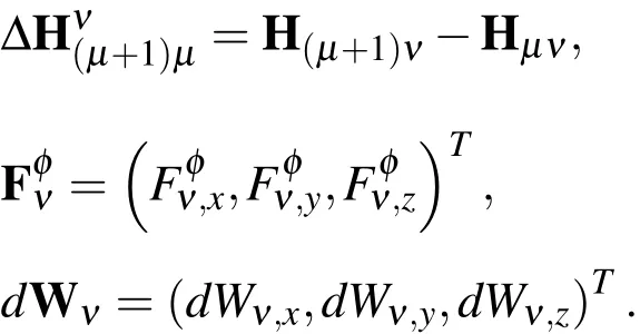
Other parameters are defined as before.The discretisation of equations(50),(51)and(52)are carried out through two interlaced procedures of different scales as presented in section 5.4.

6.1.1 Discretisation of the macro-scale governing equation

Applying the Crank-Nicolson scheme for time discretisation of the macroscopic governing equation(50)yields

or

where∆tis uniform time step;β =Re/∆t;α =0.5(1-ε);andut+1=u(y，(t+1))withu0=u(y，0).

6.1.2 Discretisation of the micro-scale stochastic governing equation

The equations in Eq.(51)are discretised using the Euler explicit scheme withNf=1024 realizations of each random process as follows.

wheretis the time level.The velocity field of the flow at the timetis given by either the initial conditions or the solution of the macro-scale procedure which was previously determined using the 1D-IRBFN method.The stress τpis then calculated using the coupling equation(52).

6.2 Creeping flows of viscoelastic fluid using FENE BSC models

This problem was solved by Koppol,Sureshkumar,and Khomami(2007)with the Reynolds numberRe=0 using the FENE-BSC model ofNS=1，3，6-dumbbell chains and neglecting HI and EV effects.The parameters of the BSC model fluid include:the ratio of polymer viscosity and total viscosity of the fluid ε=0.5,the square of maximum extensibility of the FENE dumbbell modelbD=900 and thus the square of maximum extension of each spring in the chainbBSC=bD/Ns,and the Weissenberg number of the flowWe=5.The SDE equation is developed for each dumbbell in a configuration of the 3-dumbbell BSC model as follows.

6.2.1 Temporal discretisation scheme

For microscopic procedure,the use of Euler integration scheme to discretise the SDEs in(55)yields

Based on the Euler explicit scheme,the time discretisation of Eq.(56)for dumbbell 1 is written as follows.

For the creeping problem(Re=0),the pseudo-time scheme is used to discretise the momentum conservation equation with time step size∆t=0.001 for both the micro and macro procedures.With a coarse spatial discretisation ∆y=0.1(Ny=11)and number of chainsNf=1024 at each collocation point,the numerical solutions obtained by the present method confirm a very good agreement with the results where finer meshes were used in Koppol,Sureshkumar,and Khomami(2007),evidenced by the following

•Fig.3 describes evolutions of the velocity at four locationsy=0.2,0.4,0.6 and 0.8 of the BSC models of 1,3 and 6 dumbbells.The evolution of the velocity profile indicates that the overshoots before reaching the steady state are not significant.The results show that the method is able to achieve a very high accuracy using a coarse grid(Ny=11,∆t=0.001);

•Fig.4 depicts the evolution of the first normal stress(Upper figure)and the shear stress(Lower figure)at the locationy=0.8 for several BSC models of 1,3 and 6 dumbbells using 1024 and 2048 configurations at each collocation point.The absolute values of shear stresses reach a stable stage around 0.42 to 0.48 while the stable first normal stresses cover a range from 3.2 to 4.Theses results are in very good agreement with ones in Fig.3 presented in Koppol,Sureshkumar,and Khomami(2007);

•Fig.5 shows the evolution of the first normal stress difference(Upper figure)and the square of end-to-end distance of chain configuration(Lower figure)at the locationy=0.8 for the different BSC models of 1,3 and 6 dumbbells.Several interesting points by the results for this case include:(i)the number of configurationsNf=1024 is sufficient for a reliable stochastic simulation and(ii)the more number of springs/dumbbells in a BSC model is,the higher extensibility of the BSC is.

Figure 3:The creeping planar Couette flow problem using FENE-based BSC models of 1,3 and 6 dumbbells.The parameters of the problem:number of collocation points Ny=11,Nf=1024,bD=900,We=5,ε=0.5,Re=0 and∆t=0.001.The evolution of the velocity at four locations y=0.2,y=0.4,y=0.6 and y=0.8.

Figure 6 depicts the evolution of the convergence measure of the velocity field using the FENE-based BSC model of 1,3 and 6 dumbbells by the present IRBFBCF collocation method.While most published results confirmed that convergence measures obtained for a stochastic approach are not high(from 1E-2 to 1E-3 for velocity and stress[Laso and Ottinger(1993);Tran,Mai-Duy,Le-Cao,and Tran-Cong(2012)]),the results in Fig.6 show that the convergence measure has been significantly enhanced by the present method.Furthermore,the statistical errors obtained at the steady state show a significant improvement by the present method as described in Table 1.Indeed,in most of the cases,exceptNs=3 withNf=1024,the statistical errors by the present method are smaller than those of Koppol,Sureshkumar,and Khomami(2007).

6.3 Comparisons between the Rouse and Zimm models

In this section,the difference in dynamic behaviour of dilute polymer solution in shear flow using the Rouse and Zimm models is discussed.While both of them are Hookean dumbbell-based BSC models,only the Zimm model takes into account the effect of HI.The SDE(26),describing the evolution of the configuration in dimensionless form,is rewritten for the Rouse model as

Figure 4:The creeping planar Couette flow problem using the FENE-based BSC model of 1,3 and 6 dumbbells.The parameters of the problem are given in Fig.3.The evolution of the first normal stress(Upper figure)and the shear stress(Lower figure)at location y=0.8.

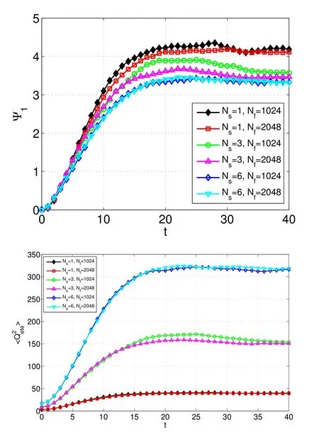
Figure 5:The creeping planar Couette flow problem using the FENE-based BSC model of 1,3 and 6 dumbbells.The parameters of the problem are given in Fig.3.The the evolution of first normal stress difference(Upper figure)and the square of end-to-end distance of the BSC configuration(Lower figure)at location y=0.8.

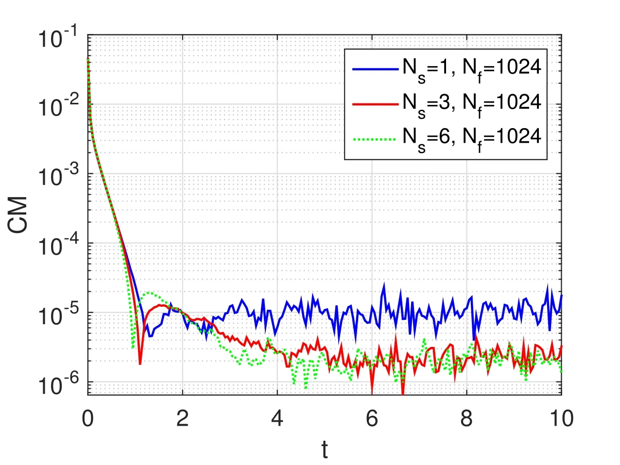
Figure 6:The creeping planar Couette flow problem using the FENE-based BSC model of 1,3 and 6 dumbbells.The parameters of the problem are given in Fig.3.The convergence measures for the velocity field are significantly enhanced in comparison with other published results.

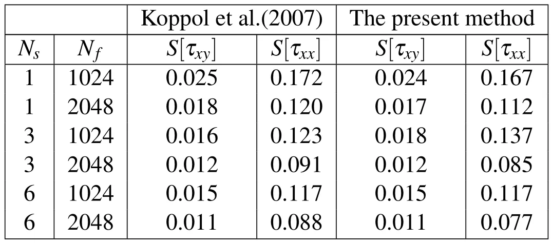
Table 1:The creeping planar Couette flow problem using the FENE-based BSC model of 1,3 and 6 dumbbells.The parameters of the problem are given in Fig.3.An evaluation on the numerical stability of the present method:the statistical errors of the shear stress and the first normal stress of the present method are compared with those of Koppol,Sureshkumar,and Khomami(2007).S[τxy]and S[τxx]are the statistical errors of the shear stress and the first normal stress,respectively.

where µ=iandare entries of the Rouse matrix of dimensionNs×Nsand given by

and for the Zimm model by

The polymer stresses are given by

whereNbandNsare the numbers of beads and springs,respectively.Other parameters are defined as before.

The start-up problem of the Rouse and Zimm models is analysed using 2-dumbbell chains with the following physical parameters:ηo=ηs+ηp=1，ρ =1.2757，λH=49.62，ηs=0.0521 as done in Laso and Ottinger(1993);Tran-Canh and Tran-Cong(2004)where ηo,ηs,ηp,ρ,are defined above.

The corresponding Weissenberg number,Reynolds number and the ratio ε are given by

Since the Zimm model takes into account the HI effect,the mechanical behaviours are significantly different from those in the Rouse model and that is shown in numerical results by the present method.Results clearly showed that the maximum extension of BS chains of the two models increases monotonically with respect to time and the increment rate of Zimm chains is higher than the Rouse ones because of the HI effect(Fig.7).Indeed,BS chain lengths reach the values of 800 and 1000 after the elapsed timet=25 for the Rouse and Zimm models,respectively.

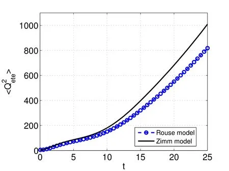
Figure 7:The start-up planar Couette flow problem using the Rouse and the Zimm models.The parameters of the problem:number of configurations Nf=1024,number of springsNs=2,the hydrodynamic interaction parameter for Zimm model=0.25,number of collocation points Ny=11,Re=1.2757,We=49.62,ε=0.9479 and∆t=0.001.The evolution of the square of end-to-end distance at the location y=0.2.

Fig.8 depicts the evolution of velocity field at four locationsy=0.2,y=0.4,y=0.6 andy=0.8 by the Rouse and Zimm models.Since they are Hookean-based BS chains,the evolution of velocity profile and values of flow velocity are nearly identical(Upper figure)except a small difference during the velocity overshoot at the start-up period(Lower figure).

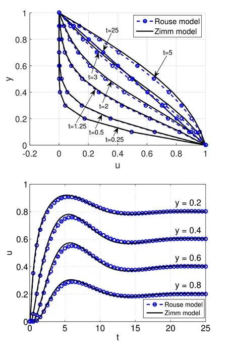
Figure 8:The start-up planar Couette flow problem using the Rouse and the Zimm models.The parameters are given in Fig.7.The evolution of the velocity profile(Upper figure)and the comparison of the evolution of velocity(Lower figure)between Rouse and Zimm models at locations y=0.2,y=0.4,y=0.6 and y=0.8.

On the rheological behaviour,the comparison between the models in the Couette start-up flows is summarised in Fig.9 for the evolution of stresses.Results in Fig.9 show that due to the HI effect,the magnitude of shear stress(Upper figure)and the first normal stress difference(Lower figure)by the Zimm model are higher than the Rouse’s ones whereas a zero-value is observed for the second normal stress differences of the two models.These results are completely in line with predictions in classical kinetic theory[Bird,Curtiss,Armstrong,and Hassager(1987);Ottinger(1996)].

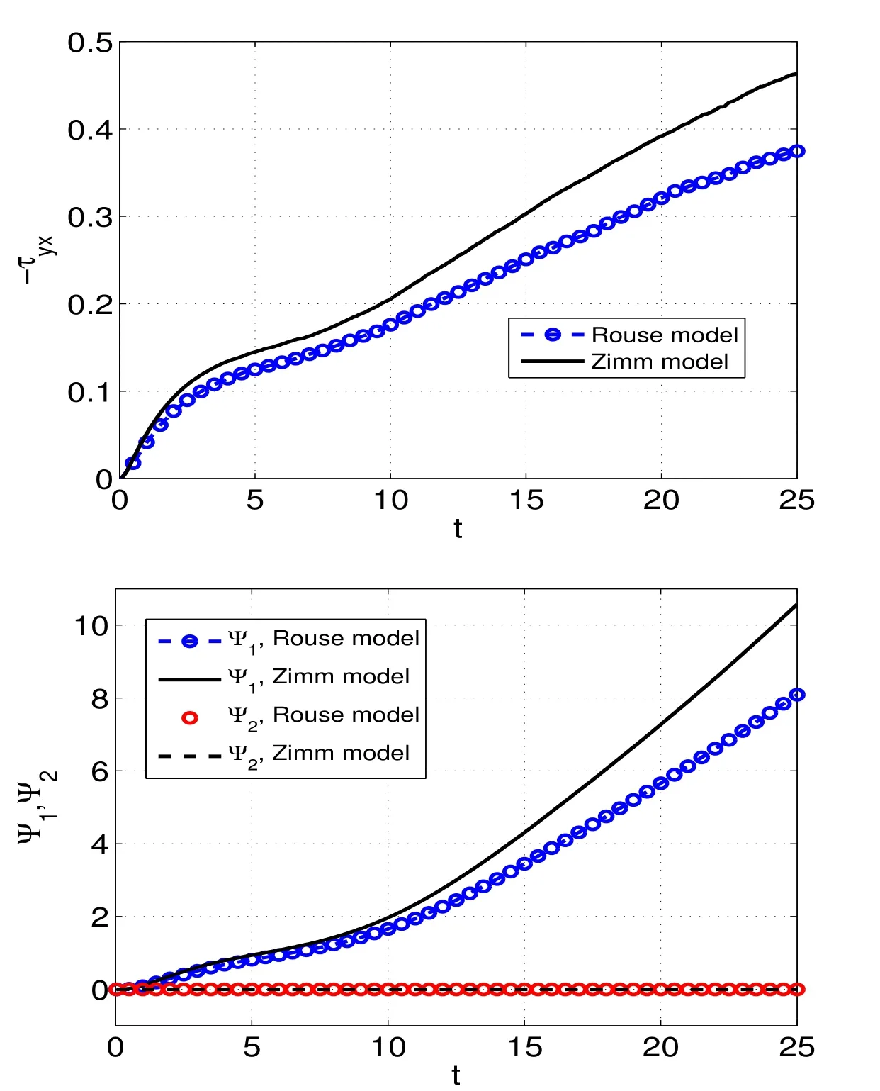
Figure 9:The start-up planar Couette flow problem using the Rouse and the Zimm models.The parameters are the same as in Fig.7.The evolution of the shear stress(Upper figure)and the evolution of the first and the second normal stress differences(Lower figure)at location y=0.2.

The simulation is also carried out with a range of Weissenberg numbers(We=5,10 and 30)to investigate the present method.Results presented in Figs.10 and 11 confirm the influence of the Weissenberg number on the velocity through the start-up period,the shear stress and the first normal stress difference.

For the evolution of velocity,Fig.10 shows that the maximum amplitude as well as the oscillatory frequency of the over/undershoot are higher for smaller Weissenberg numbers for both Rouse and Zimm models.Meanwhile,with a given Weissenberg number,due to the HI effect,the over/undershoot of velocity is stronger with the Zimm model.

On the polymer stresses,the higher Weissenberg number is,the lower magnitude of the shear stress(Fig.11-Upper figure)and the first normal stress difference(Fig.11-Lower figure)are for both Rouse and Zimm models.Furthermore,with a given Weissenberg number,the absolute value of shear stress and the first normal stress difference of flow by the Zimm model are higher than those by the Rouse model.

Figure 10:The start-up planar Couette flow problem using the Rouse and the Zimm models.The parameters are the same as in Fig.7.Comparison of the fluid rheological properties using the Rouse and Zimm models for several Weissenberg numbers(We=5，10 and 30).The evolution of velocity.

Figure 11:The start-up planar Couette flow problem using the Rouse and the Zimm models.The parameters are the same as in Fig.7.Comparison of the fluid rheological properties using the Rouse and Zimm models for several Weissenberg numbers(We=5，10 and 30).The evolution of the shear stress(Upper figure)and the first normal stress difference at location y=0.2(Lower figure).

6.4 Start-up Couette flow using the FENE-based BSC models with HI and EV effects

The method is finally demonstrated with the start-up Couette flow of fully nonlinear FENE-based BSC model fluids.The HI and EV effects are included in the model with varying number of FENE dumbbells in each chain(Ns=1，2，···，6).The governing SDE(26)of a general BSC model with HI and EV effects and the extra stress formula for the polymer(27)are reproduced as follows.

where Z is determined by Eq.(30)and other parameters are defined as before.

The physical parameters of the fluid,including the Weissenberg number,Reynolds number and the ratio ε,are chosen as presented in section 6.3.The parameters¯h=0.25 for the HI effect and the constantsz=1(Eq.(17))andK=1(Eq.(18))for the EV effect are used in this section.

On the mechanical behaviour,Fig.12 depicts the evolution of shear stress and Fig.13 the first normal stress difference(Upper figure)and the second normal stress difference(Lower figure)at the location ofy=0.2.Overshoots are observed for shear stress,the first and the second normal stress differences.In particular,the existence of the non-zero second normal stress difference is very clear as compared with simulations using the BSC models without both HI and EV effects(see cases of Rouse and Zimm models in Fig.9-Lower figure).This is because the nonlinear effects of HI and EV have been included in the simulations.Results also show the influence of the number of dumbbells in a polymer chain on the dynamics properties through the start-up time before reaching stable values.For example,the overshoot of the shear stress(Fig.12)and the first normal stress difference(Fig.13-Upper figure)decrease with increasing number of dumbbells in the chain configuration.

The development of velocity with respect to time at different locations(y=0.2,0.4,0.6 and 0.8)are presented in Fig.14.Generally,an overshoot at the beginning time is formed before a stable state is reached.The obtained results show a significant influence of the number of dumbbells in the chain on the initial transient behaviour.It can be seen clearly that the velocity simulated with higher number of dumbbells achieves the maximum value(or the debut position of the overshoot)sooner and thus needs less time to reach stable state(Lower figure).

Last but not least,it is worth noting that with a givenbD,the HI and EV influences on the polymer stresses increase and only significantly for polymer chains having large enough number of dumbbells in chain(Fig.15).For example,the difference of the shear stress(Upper figure)and the first normal stress difference(Lower figure)of the FENE-BSC models with and without HI and EV are very small for the 2-dumbbell chain model but very significant for the 6-dumbbell chain model.A similar observation can be seen for the square maximum extension of end-to-end connecting vector(Fig.16).Meanwhile,these nonlinear effects are not significant for the velocity field of the flow(Fig.17).

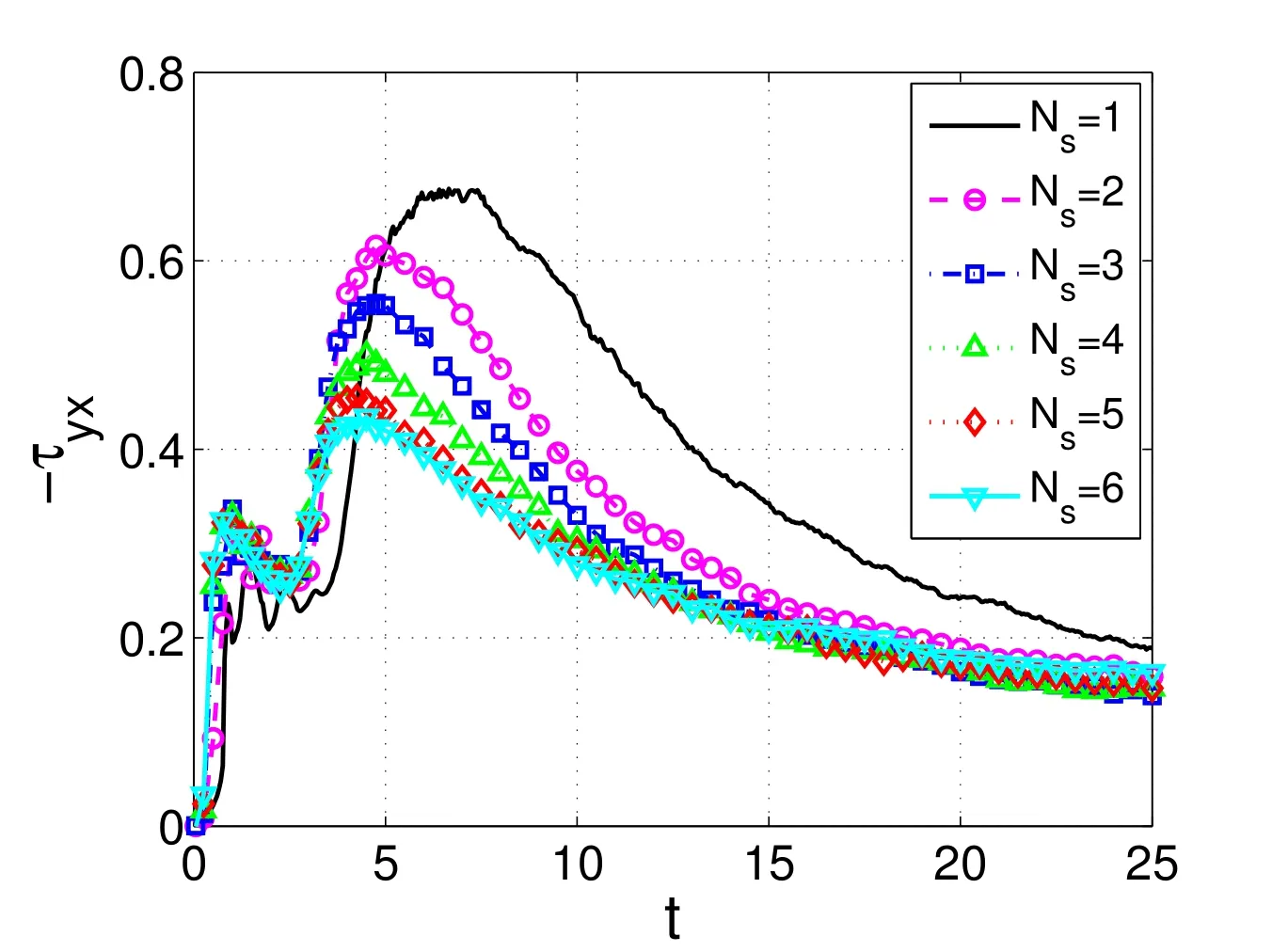
Figure 12:The start-up planar Couette flow problem using FENE-based BSC models of several numbers of dumbbells with HI and EV effects.The parameters of the problem:¯h=0.25,z=1,K=1,Ny=11,We=49.62,ε=0.9479,bD=50.The evolution of the shear stress at location y=0.2 using 1，2，3，4，5 and 6 dumbbells.

Figure 13:The start-up planar Couette flow problem using FENE-based BSC models of several numbers of dumbbells with HI and EV effects.The parameters are the same as in Fig.12.The evolution of the first normal stress difference(Upper figure)and the second normal stress difference(Lower figure)at location y=0.2 using 1，2，3，4，5 and 6 dumbbells.

Figure 14:The start-up planar Couette flow problem using FENE-based BSC models of several numbers of dumbbells with HI and EV effects.The parameters are the same as in Fig.12.The evolution of the velocity field at locations y=0.2,y=0.4,y=0.6 and y=0.8(Upper figure)and an enlarged velocity profile at location y=0.6(Lower figure)using 1，2，3，4，5 and 6 dumbbells.

Figure 15:The start-up planar Couette flow problem using FENE-based BSC models of several numbers of dumbbells.The parameters are shown as in Fig.12.The influence of HI and EV effects on rheological properties of the fluid.The evolution of the shear stress(Upper figure)and the first normal stress difference(Lower figure)at location y=0.2.

Figure 16:The start-up planar Couette flow problem using FENE-based BSC models of several numbers of dumbbells.The parameters are shown as in Fig.12.The influence of HI and EV effects on rheological properties of the fluid.The evolution of the end-to-end connector vector at location y=0.2.

Figure 17:The start-up planar Couette flow problem using FENE-based BSC models of several numbers of dumbbells.The parameters are shown as in Fig.12.The influence of HI and EV effects on rheological properties of the fluid.The evolution of the velocity pro file with/without EV and HI effects using 2-dumbbell(Upper figure)and 6-dumbbell(Lower figure)BSC models at locations y=0.2,y=0.4,y=0.6 and y=0.8.

6.5 Performance of Parallel computation

The problem is solved using 1024 BSCs at each collocation point to ensure the accuracy and stability in stochastically determining the stresses.In order to estimate the efficiency of the parallel algorithm,a range of 2,4 and 8 CPUs is used to solve the SDEs corresponding to 1024 configurations in parallel generated at each and every collocation point and to determine the averaged stresses at the grid points.Especially,the presence of HI and EV effects makes a massive increase in the computational cost because of the bead-bead and bead-spring interactions in the fluid model.For this numerical example,the FENE-BSC model of 2 dumbbells with HI and EV effects is considered to initially evaluate the efficiency of the parallel algorithm.

Table 2 shows the effect of the number of CPUs on the speed-up as well as the efficiency of the parallel technique.A significant improvement of the throughput has been achieved.For example,the speed-up increased 1.7,2.96 and 3.66 times when using 2,4 and 8 CPUs,respectively.However,the efficiency of the algorithm reduces with increasing number of CPUs.The results presented in Table 2 and Fig.18 show the effect of the number of CPUs on the speed-up and the efficiency of the present method are in agreement with several recent results reported in Tran,Phillips,and Tran-Cong(2009);Laso,Picasso,and Ottinger(1997).

Table 2:The start-up planar Couette flow problem using FENE-BSC models with HI and EV effects.The parameters of problem:number of dumbbells in a BSC Ns=2,number of BSC configurations at each collocation point Nf=1024,∆t=0.001,number of iterations it=2.5E+4.Parallel computation results are shown in the table where CPUs is number of CPUs,tmis elapsed time for the micro-procedure,tMis elapsed time for the macro-procedure,S is single mode,P is parallel mode,Spd is speed-up and Eff is efficiency.

7 Conclusions

Figure 18:The start-up planar Couette flow problem using FENE-BSC models of 2 dumbbells with HI and EV effects:The parameters are shown as in Fig.12.Parallel computation results:The efficiency(Left figure)and the speed-up(Right figure)with respect to the number of CPUs.

The IRBFN-BCF based coarse-grained method is employed to simulate the flow of dilute polymer solutions using complex nonlinear BSC models.The hybrid simulation method is a combination of a high order RBFN-based approximation for the solution of macroscopic conservation equations and a BCF-based CG technique for the evolution of polymer configuration.The present method offers the advantages of a mesh-free based stochastic CG method in the simulation of viscoelastic polymer flows as presented in Tran,An-Vo,Mai-Duy,and Tran-Cong(2011).The method efficiency based on both the enhanced convergence rate of numerical solution and the stability of a stochastic process is evidenced by the successful simulation of flows using complex BSC models which take into account nonlinear interaction forces in the polymer solution,e.g.HI and EV effects.This allows the method to effectively simulate models which are realistic in comparison with experimental results.

Acknowledgement:The first author would like to thank the University of Southern Queensland for a Postgraduate Research scholarship and Scholarship Supplements by the Faculty of Health,Engineering and Sciences and the Computational Engineering and Science Research Centre.These supports are gratefully acknowledged.We would like to thank the reviewers for their helpful comments.

Bird,R.B.;Curtiss,C.F.;Armstrong,R.C.;Hassager,O.(1987):Dynamics of Polymer Liquids,V.2.John Wiley&Sons:New York.

Herrchen,M.;Ottinger,H.C.(1997):A detailed comparison of various FENE dumbbell models.Journal of Non-Newtonian Fluid Mechanics,vol.68,no.1,pp.17–42.

Hulsen,M.A.;Van Heel,A.P.G.;Van Den Brule,B.H.A.A.(1997):Simulation of viscoelastic flows using brownian configuration fields.Journal of Non-Newtonian Fluid Mechanics,vol.70,no.1,pp.79–101.

Koppol,A.P.;Sureshkumar,R.;Khomami,B.(2007): An efficient algorithm for multiscale flow simulation of dilute polymeric solutions using bead-spring chains.Journal of non-newtonian fluid mechanics,vol.141,no.2,pp.180–192.

Laso,M.;Ottinger,H.C.(1993):Calculation of viscoelastic flow using molecular models:the CONNFFESSIT approach.Journal of Non-Newtonian Fluid Mechanics,vol.47,pp.1–20.

Laso,M.;Picasso,M.;Ottinger,H.C.(1997):Two dimensional time dependent viscoelastic flow calculations using CONNFFESSIT.AIChE J.,vol.43(4),pp.877–892.

Liu,S.;Liu,X.;Guan,X.F.;He,P.F.;Yuan,Y.(2013): A stochastic multiscale model for predicting the thermal expansion coefficient of early-age concrete.CMES:Computer Modeling in Engineering and Sciences,vol.92,no.2,pp.173–191.

Liu,S.;Liu,X.;Yuan,Y.;He,P.F.;Mang,H.A.(2014):A stochastic multiscale model for prediction of the autogenous shrinkage deformations of early-age concrete.CMC:Computers Materials and Continua,vol.39,no.2,pp.85–112.

Liu,S.;Liu,X.;Yuan,Y.;Mang,H.A.;Zhang,D.-G.;Zhou,H.-M.;Yang,Q.W.;Du,S.G.;Liang,C.F.;Yang,L.J.(2014): Constitutive modeling of early-age concrete by a stochastic multi-scale method.CMES:Computer Modeling in Engineering and Sciences,vol.100,no.3,pp.157–200.

Magda,J.J.;Larson,R.G.;Mackay,M.E.(1988): Deformation-dependent hydrodynamic interaction in flows of dilute polymer solutions.The Journal of Chemical Physics,vol.89,no.4,pp.2504–2513.

Mai-Duy,N.;Tran-Cong,T.(2007): A collocation method based on onedimensional rbf interpolation scheme for solving pdes.International Journal of Numerical Methods for Heat and Fluid Flow,vol.26,pp.426–447.

Mochimaru,Y.(1983): Unsteady-state development of plane Couette flow for viscoelastic fluids.Journal of Non-Newtonian Fluid Mechanics,vol.12,no.2,pp.135–152.

Ottinger,H.C.(1987):A model of dilute polymer solutions with hydrodynamic interaction and finite extensibility.I.Basic equations and series expansions.Journal of Non-Newtonian Fluid Mechanics,vol.26,no.2,pp.207–246.

Ottinger,H.C.(1987): Generalized Zimm model for dilute polymer solutions under theta conditions.The Journal of Chemical Physics,vol.86,no.6,pp.3731–3749.

Ottinger,H.C.(1989):Gaussian approximation for Rouse chains with hydrodynamic interaction.The Journal of Chemical Physics,vol.90,no.1,pp.463–473.

Ottinger,H.C.(1996):Stochastic processes in polymeric fluids:tools and examples for developing simulation algorithms.Springer:Berlin.

Phan-Thien,N.(2012):Understanding viscoelasticity:An Introduction to Rheology.Springer-Verlag:Berlin.

Prabhakar,R.;Prakash,J.R.(2004):Multiplicative separation of the influences of excluded volume,hydrodynamic interactions and finite extensibility on the rheological properties of dilute polymer solutions.Journal of Non-Newtonian Fluid Mechanics,vol.116,no.2,pp.163–183.

Prakash,J.R.(2001): Rouse chains with excluded volume interactions:linear viscoelasticity.Macromolecules,vol.34,no.10,pp.3396–3411.

Prakash,J.R.(2002):Rouse chains with excluded volume interactions in steady simple shear flow.Journal of Rheology,vol.46,no.6,pp.1353–1380.

Rotne,J.;Prager,S.(1969):Variational treatment of hydrodynamic interaction in polymers.The Journal of Chemical Physics,vol.50,pp.4831–4837.

Rouse,J.;Prince,E.(1953): A theory of the linear viscoelastic properties of dilute solutions of coiling polymers.The Journal of Chemical Physics,vol.21,no.7,pp.1272–1280.

Sunthar,P.;Prakash,J.R.(2005):Parameter-free prediction of dna conformations in elongational flow by successive fine graining.Macromolecules,vol.38,no.2,pp.617–640.

Tran,C.D.;An-Vo,D.A.;Mai-Duy,N.;Tran-Cong,T.(2011): An integrated RBFN-based macro-micro multi-scale method for computation of viscoelastic fluid flows.CMES:Computer Modeling in Engineering and Sciences,vol.82,no.2,pp.137–162.

Tran,C.D.;Mai-Duy,N.;Le-Cao,K.;Tran-Cong,T.(2012):A continuummicroscopic method based on IRBFs and control volume scheme for viscoelastic fluid flows.CMES:Computer Modeling in Engineering and Sciences,vol.85,no.6,pp.499–519.

Tran,C.D.;Phillips,D.G.;Tran-Cong,T.(2009):Computation of dilute polymer solution flows using BCF-RBFN based method and domain decomposition technique.Korea-Australia Rheology Journal,vol.21(1),pp.1–12.

Tran-Canh,D.;Tran-Cong,T.(2002):Computation of viscoelastic flow using neural networks and stochastic simulation.Korea-Australia Rheology Journal,vol.14,no.4,pp.161–174.

Tran-Canh,D.;Tran-Cong,T.(2004):Element-free simulation of dilute polymeric flows using Brownian Configuration Fields.Korea-Australia Rheology Journal,vol.16,no.1,pp.1–15.

Wedgewood,L.E.;Ostrov,D.N.;Bird,R.B.(1991): Kinetic theory and rheology of dilute suspensions of finitely extendible dumbbells.Journal of Non-Newtonian Fluid Mechanics,vol.40,no.1,pp.119–139.

Wiest,J.M.;Tanner,R.I.(1989): Rheology of bead-nonlinear spring chain macromolecules.Journal of Rheology,vol.33,no.2,pp.281–316.

Yamakawa,H.(1971):Modern theory of polymer solutions.Happer and Row:New York.

Zimm,B.H.(1956): Dynamics of polymer molecules in dilute solution:viscoelasticity,flow birefringence and dielectric loss.The Journal of Chemical Physics,vol.24,pp.269–278.

Zylka,W.(1991):Gaussian approximation and Brownian dynamics simulations for Rouse chains with hydrodynamic interaction undergoing simple shear flow.The Journal of Chemical Physics,vol.94,no.1,pp.4628.

1Computational Engineering and Science Research Centre,Faculty of Health,Engineering and Science,The University of Southern Queensland,Toowoomba,QLD 4350,Australia.