Prouhet-Thue-Morse sequence and atomic functions in applications of physics and techniques

Victor F Kravchenko, Oleg V Kravchenko,3, Yaroslav Y Konovalov

(1. Kotelnikov Institute of Radio-engineering and Electronics, Russian Academy of Sciences, Moscow 125009, Russia;2. Bauman Moscow State Technical University, Moscow 105005, Russia;3. Scientific and Technological Center of Unique Instrumentation, Moscow 117342, Russia)



Prouhet-Thue-Morse sequence and atomic functions in applications of physics and techniques

Victor F Kravchenko1,2, Oleg V Kravchenko1,2,3, Yaroslav Y Konovalov2

(1.KotelnikovInstituteofRadio-engineeringandElectronics,RussianAcademyofSciences,Moscow125009,Russia;2.BaumanMoscowStateTechnicalUniversity,Moscow105005,Russia;3.ScientificandTechnologicalCenterofUniqueInstrumentation,Moscow117342,Russia)

In present article a number of results are described in a systematic way concerning both signal and image processing problems with respect to atomic functions theory and Prouhet-Thue-Morse sequence.

atomic functions; Prouhet-Thue-Morse sequence; digital signal processing; image processing

0 Introduction

The famous Prouhet-Tarry-Escott (PTE) problem[1]seeks collections of mutually disjoint sets of nonnegative integers having equal sums of the same powers. The PTE problem is as follows:

LetS={0,1,…N-1}. GivenM, is it possible to partitionSinto two disjoint subsetsS0andS1such that

for all 0≤m≤M?

Prouhet-Thue-Morse (PTM) sequence was first studied by Eugene Prouhet in 1851 who applied it to number theory. However, Prouhet did not mentioned the sequence explicitly. This was left to Axel Thue in 1906， who used it to find the study of combinatories on words. The sequence was only brought to worldwide attention with the work of Marston Morse in 1921 when he applied it to differential geometry. The sequence has been discovered independently many times not always by professional research mathematicians. For example, Max Euwe, a chess grandmaster who held the world championship title from 1935 to 1937 and mathematics teacher, discovered it in 1929 in an application to chess as an example of an infinite chess game. The PTM sequence is usually defined as a sequence of “1” and “0” in number theory, as “A” and “B” in physics of quasycrystalls, and “1” and “0” in signal processing as well.

Let us define a PTM sequence in such a way:t(1)=1 by definition. Then if the segment of the length 2nis constructed, we will continue it with the same one with signs of all terms changed to anothert(2n+k)=-t(k) for all 1≤k≤2n. The first 8 terms of the sequence are

The PTM sequence[2]is a well-known self-similar sequence applied in coding, cryptography, etc. It has a strong connection with a PTE problem, and a simple proof of PTE has been introduced recently with the usage of the PTM sequence[3].

Not so far a simple way of arithmetic and logic unit construction without multiplies on adders only was introduced by Wolfgang Hilberg in a patent[4]. The main advantage of the developed method is that it implies an integer arithmetic only to encode logical one or zero. The fractal property as a self-similarity of continuous analog of PTM sequence (known ashut(x) orup(x) function) was also used to develop a simple technique for compensation of Doppler effects which was introduced by Todor Cooklev in Ref.[5]. This property as a property of symmetry allowed reducing operations in digital device at least in two times.

PTM ordering (so called P8 sequence) was also used as the first five Walsh functions (Paley ordering) in switched observations at the 12 Meter Telescope[6]. Such a property was also employed in the vertical receiver device which was mentioned to solve the problem of offshore hydrocarbon exploration[10].

Then, the PTM sequence was used to develop an efficient optimization algorithm of a complex system management by Viktor Korotkikh[7]. While choosing the next strategy for each agent, one should follow an optimal fuzzy if-then rule on the basis of the PTM sequence:

1) If the last strategy is successful, then continue with the same strategy.

2) If the last strategy is unsuccessful, then ask PTM generator.

Thestructureofthereviewisinthefollowing.Inthenextsection,wewillconsideranabstractmathematicalproblemofconstructionoflineartimeinvariant(LTI)systemwithbothPTMinputandoutput.Then,wewillconsideralinkbetweeninfinitelydifferentialcontinuousatomicfunctionsandthePTMsequence,anddescribesomegeneralizationsofthealgorithmbyWolfgangHilbergtoresolveacorrespondingfunctional-differentialequation.Intheendwewilldiscusssomephysicalmodelswhichallowustofindanaivetheorywithphysicalmeaningoftheatomicfunctionsaswell.

1 LTI PTM system

Withrespecttothedigitalsystems,let’sconsideradiscreteLTIsystemwithhnimpulsecharacteristicandletxnbeinputdiscretesequence.Forexample,therearefirst4elementsofthePTMsequence

Inthegeneralcase,thelengthofxnsequenceislx,lengthofsequenceynisly,andthelengthofhnisln.SinceLTI’sinputisxn,theLTI’soutputwillbedefinedbytheconvolution

yn=xn*hn.

Themathematicalquestionis:willweobtainthePTMoutputynunderunknownhnwithzeromean?

Let’sdescribehowtoobtainthePTMoutput.It’sobviousthatthelengthynisdefinedbylxandlh,

(1)

Considertheparticleexampleofthisproblem.Let’skeepthelengthofinputxnaslx=4.Inthiscase

Thenwewillhave

IfwehavetoobtainthePTMoutputynwithlengthly=2lx=8withtheelements

Thenthelengthofhnwillbelh=ly-lx+1=5.

(2)

Eq.(2)willhavethefollowingmatrixform:

(3)

Onecouldshoweasilytherankrank(Alb)=rank(A)=5,thenthereisanontrivialsolutionofEq.(3)suchas

(4)

(5)

(6)

WecanalsofindthePTMpattern(4)inEq.(6).Forexample,

Table 1 Connection between the lengths of xn, yn and hn

Let’s consider a deep connection between the PTM and atomic functions as products of similar iterative procedures of corresponding PTM sequences. It allows us to conduct an investigation of the properties of atomic functions (AFs) based on the properties of PTM and conversely. Native application of this connection is a construction of fast iterative algorithms for computation of AFs. Another interesting effect of it is appearance of functions similar to atomic ones in the problem with PTM coefficients.

2 Atomic functions and iterative algorithms

AFs[11-14]were introduced in 1971 by V L and V A Rvachevs. The first and most known AFup(x) was constructed as a solution of the next problem. The derivative of compactly supported hump-like function consists of the hump and the pit. Is there a function whose hump and pit are similar to the hump of the function? If we set the support of the unknown function to [-1,1], the problem can be represented as a functional-differential equation (FDE)

(7)

Applying Fourier transform to the FDE, one can find that the solution exists, and ifa=2, the spectrum of the solution can be obtained as an infinite product of compressed sinc(ω) functionsω(Fig.1(b))

(8)

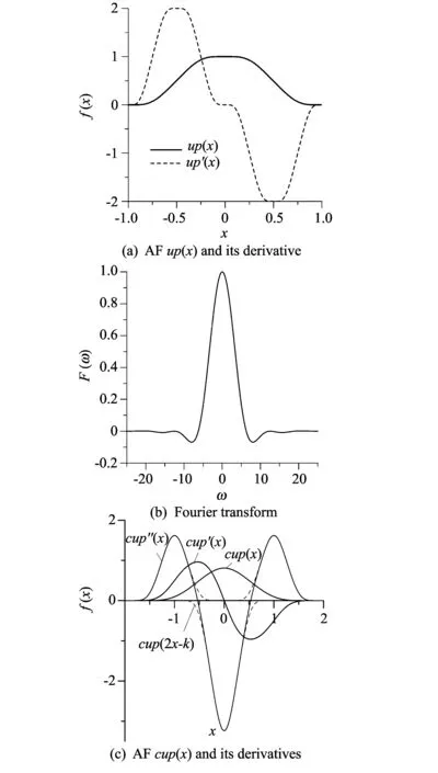
Fig.1 AF up(x), cup(x) and their derivatives

The solution of Eq.(1) can be presented as a sum of corresponding Fourier series (Fig.1(a)):

(9)

In the general definition AFs are compactly supported solutions of FDEs presented in the form

(10)

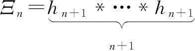
whereL(f) is a linear differential operator, and usuallyL(f)=f(n). The most important AFs areha(x),fupn(x),Ξn(x), andcup(x) function (Fig.1(c)).

Looking atn-time derivative of AFup(x) one can find that it consists of humps and pits ordered like “1” and “-1” in PTM. To prove this property, note thatup(0)(x)=up(x). It is a hump which can be represented as “1” in PTM. Then according to Eq.(10)

(2up(2x+1)-2up(2x-1))(n)=

2up(n)(2x+1)-2up(n)(2x-1).

It means thatup(n+1)(x) consists of compressedup(n)(x) continued with -up(n)(x). This procedure is similar to the iterative procedure of the PTM construction described above. The signs of the terms ofn-time derivative are ordered as PTM, andn-time derivative ofup(x) can be presented as

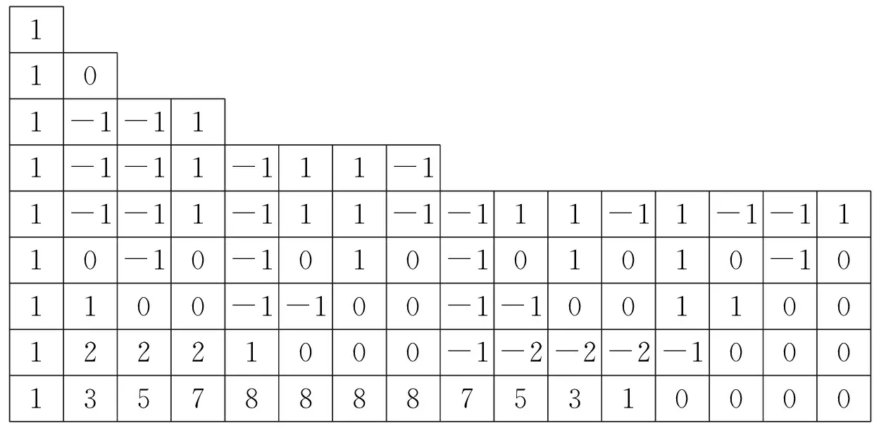
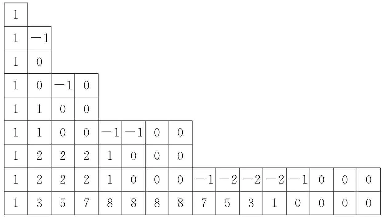
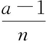
wheretkare terms of PTM. Another way to solve the FDE (7) was presented in Ref.[4] by Wolfgang Hilberg. It looks like a trick. Let’s construct a segment of the PTM sequence with the length 2n. Aftern-time summation and normalization, we will obtain 2npoints ofup(x) function. This method is demonstrated in Table 2(a).

Table 2 Computation ofup(x) according to Ref.[4](a) and by iterative method (b)

1101-1-111-1-11-111-11-1-11-111-1-111-11-1-1110-10-1010-101010-101100-1-100-1-100110012221000-1-2-2-2-10001357888875310000

(a)

(b)

TheyareAFstooandsatisfytheequations:

(11)

An effective iterative algorithm for computing all of these functions is presented in Refs.[15]-[17]. Two AFsf(x) andg(x) with the same scale parameteraand the equations are constructed as

(12)

(13)

(14)

(15)

Multiplication of Eqs.(14) and (15) gives equation for product in the following form:

(16)

A reverse Fourier transform according to

gives the equation for the convolutionh(x)=f(x)*g(x),

(17)

Eq.(17) is a special case of Eq.(10), therefore,h(x) is an atomic function indeed. Afterwards, an iterative algorithm is constructed for computing the convolutionh(x). It consists of the next two steps repeated while required accuracy is not achieved: construction of the sequence with structure based on the form of right-hand part of Eq.(17) and its summationnf+ngtimes. Here are some examples.

Example 1 The first example is an itself convolution ofha(x) function:ha(x)*ha(x). Applying Eq.(17), we obtain

(18)

The convolution function ofha(x)*ha(x) witha=4 is shown in Fig.2.

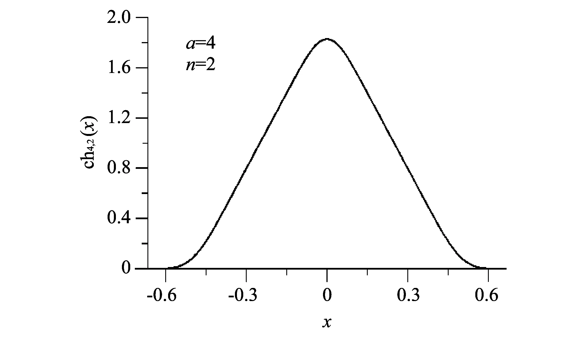
Fig.2 Convolution AF h4(x)*h4(x)

Example 2 The second example is a convolutionupm(x)*ha(x). Consider the convolution ofupm(x) withha(x), where the atomic functionupm(x) satisfies the equation

(19)

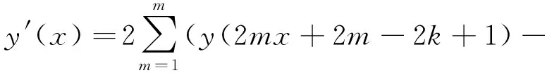
Let the scale parameters of the equations are equal (a=2m). Applying Eq.(17) to the previous equation, we obtain

y(2mx+2m-2k)-y(2mx-2k+2)+

y(2mx-2k)).

After opening brackets, we get a short and clear equation for the convolutionupm(x)*h2m(x) as

y(x)=2m(y(2mx+2m)-y(2mx)+

y(2mx-2m)).

Eq.(11) is a special case of constructed equation withm=1.

After some considerations, a two-parameter family of atomic functions which is presented as cha,ncan be introduced. In Example 1, the equation for the convolutionha*hais constructed. Based on its triple convolution,ha*ha*ha=(ha*ha)*hacan be considered, then the quadruple convolutionha*ha*…*ha*ha=(ha*ha*ha)*ha, etc.

We define a new two-parameter family of functions cha,nas the convolution[17]

Doing the iterative procedure as Eq.(17) byn-1 times, we obtain FDE for the constructed functions,

(20)

wherea>1 andn=1,2,3,…. Enumerated in the introduction of AFs are the special cases ofcha,nwith the fixed values of the parameters,

Familycha,n(x) allows investigating the properties of AFs in an unified way(see Table 3). Consider some properties of the new family of AFs.

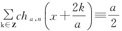
Table 3 Supports of terms of right-hand part of equation of cha,n(x)

Shifts ofcha,ngive a constant decomposition as follows:

An exact decomposition of any polynomial degree less or equal ton-1, is given by

The property allows the construction of effective interpolation of smooth functions. Examples of 1D and 2D interpolations and their applications to solving the boundary-value problems are presented in Ref.[17].

4) Based on Eq.(20), recurrent formulas for even momentscha,n(x) are constructed. View of the formulas depends onn. Forn=2 andn=3, we have, respectively

Note that according to the above definition, the function discussed in Example 1 ischa,n.

3 Iterative computation of AFs

Considerup(x) as a fixed point of contraction operator

(21)

According to the contraction mapping principle,up(x) is limit of the sequence {fn(x)} withfn+1(x)=A(fn). There are generally three ways of practical construction of the sequence {fn(x)}: analytical construction, numerical integration and summation of self-similar sequences.

The first way means analytical computation of integral as Eq.(21) to obtain convergent sequence of interpolations of AFup(x). With the starting pointf0(x)≡0.5, it provides a sequence of splines of increasing degree. These splines are called perfect splines. To obtain good accuracy, one has to consider splines of high degree. Then perfect splines are not convenient for practical calculation. In the second way, analytical transforms are replaced with numerical computation of integrals as Eq.(21). This method is clear and can be performed for any FDE with any right-hand part. The main disadvantage of this method is accumulation of the computation error at the right end of the integration segment. This error can lead to distortion of function, spoiled its symmetry and even break convergence of the algorithm. The third way is summation of special self-similar sequences. This method is similar to the previous one, but all computation is performed on integer numbers without accumulation of computation error. This method provides successive approximations with step functions considered as sequences. In terms of the sequences the operatorA(f) forup(x) function can be represented as composition of two steps: continuation of constructed segment of the sequence with the same one with reversed signs of terms and summation of the sequence corresponding to the integration in operatorA(f). The example of computation with starting point is shown in Table 1(b). It is clear that Hilberg’s method described above is similar to the iterative method with another order of computation. Giving the same result, the iterative method requires less arithmetical operations than Hilberg’s. For any other FDE, a similar iterative method can be constructed. It will be presented as iterated composition of two steps: continuation of the sequence according to the right-hand part of equation and iterated summation corresponding to the integration in operatorA(f). Then each AF corresponds to the self-similar sequence constructed according to the right-hand part of equation.

Here, AFcup(x) (See Fig.1(c)) as an example of the construction of the iterative algorithms is discussed. It is known[13]that the convolutions of AFs are AFs too. Thencup(x)=up(x)*up(x) is an AF with the support [-2,2] and the equation

y″(x)=2y(2x+2)-4y(2x)+2y(2x-2).

The supports of the terms of right-hand part of FDE are respectively [-2,0], [-1,1] and [0,2]. The terms are intersected and each term is shifted from one another on the half of its length. Then corresponding continuation operation can be described as in the following. If some segment of the sequence is constructed, a new segment of double length consists of three segments similar to be shifted from each other to the half of their lengths multiplied by the coefficients 1, -2 and 1 according to the right-hand part of the equation. Then this new sequence must be summated two times since the FDE is of second order. In Table 4,cup(x) function, its derivatives and examples of iterative computation are shown.

Table 4cup(x) function and its iterative computation

The main advantage of these iterative algorithms is that they allow very fast and accurate computation of AFs and their convolutions. A general description of the iterative approach to the computation of AFs is given in Refs.[15]-[17].

According to Eq.(21), consider the following more general self-similar operator,

(22)

OperatorA(y) consists of two steps: summation of the terms of the right-hand part of Eq.(20) and integration ofntimes.

Depending on the method of integration, there are three different ways of practical construction of the sequence.

1) Analytical calculation of integrals. With starting point

It provides a sequence of splines of increasing degree.

2) Numerical computation of integrands. This method is clear and can be simply performed for FDE with any right-hand part. The main disadvantage of this method is accumulation of the computation error at the right end of integration segment. This error can lead to distortion of the function, spoiled symmetry and even break convergence of the algorithm.

3) Summation of special self-similar sequences. This method is similar to the previous one, but all computation is performed on integer numbers without accumulation of the computation error. This method provides successive approximations with step functions considered as a sequence.

Let us discuss the third way of iterative computation.fkis presented as a sequence with lengthlk. OperatorA(y) is a composition of two operations: addition terms of the right-hand part of the equation and n-times integration. The first operation is presented as construction of the new sequence with lengthlk+1from the shifted segments of the previous one. The second operation is a summation of the sequence performedntimes.

Table 5 Computation of ch3,3(x) function

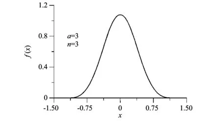
Fig.3 Function ch3,3(x)

Then we apply the operator to it. The first step of the operation is addition to the segment of the previous sequence of the two same segments multiplied respectively by -2 and 1. The terms are shifted from each other with 3 points. The empty space is filled by zeros. We obtain a new sequence with quadruple length. Then we integrate this sequence two times. We repeat the steps to achieve the required accuracy. The example of the computation is shown in Table 6. The graph of the function is presented in Fig.2.

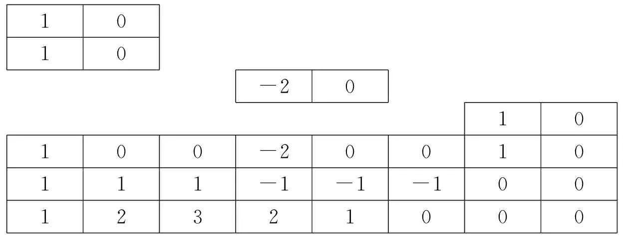
Table 6 Computation of ch4,2(x) function

Notethatatomicfunctionsareevenandsymmetricandtheirincreasinganddecreasingintervalsareinthesamescale.ThesepropertiesmakeitpossibletouseFourierseriesfortheircomputation.InthecaseofmorecomplicatedstructureofFDEitmaybemoredifficultorimpossibletousetheFouriermethod.However,theiterativealgorithmallowsfindingthecompactlysupportedsolutionsofsuchFDEs.Inthereport,examplesofapplicationofalgorithmaredemonstratedtothefollowingcases:

i)Thefunctionisnotsymmetric(increasinganddecreasingintervalsalternateinanyarbitraryorder).

Example3FDEisthefollowing,

ii) Increasing and decreasing intervals are in different scales (akin Eq.(10) are different).

Example 4 Two FDEs are as follows:

Examples of the work of the algorithm are presented in Figs.4(a)-(c). Implementation of some AFs can be found in Ref.[20] and implementation of the iterative algorithm ofup(x) approximation via the PTM sequence[6]can be found in Ref.[19] as well.

Fig.4 Solutions of FDEs

4 PTM sequence and physical models

It seems to be unclear to ask about some ideas behind the physical interpretation of the functional differential equations like Eq.(10) and their finite solutions likeup(x).

The native consequence of the previous considerations is that Eq.(10) may appear in some situations when the PTM sequence arises in some media. So, let us consider a so-called PTM chain.

Let us have the sequence of masses {mj},j=1,…,Nis such that the indices 0 and 1 are distributed according to the PTM sequence joined by the springs with stiffnessk(Fig.5). The name of such kind of structure is “quasy-alloy” by analogy with quasicrystal models (like Fibonacci quasicrystal models). A detailed reference about this question can be found in Ref.[16].

So, when we consider a tight-binding model of atoms like in Fig.5 with site energies arranged in the PTM sequence, we have a transfer matrix

(23)

The typical situation is presented in Figs.6(a) and (b). It is a fractal-like wavefunction which is computed by Eq.(23) with the initial condition:ψ1=1,ψ2=3,V0=1,E=1,723 817 824 andN=213(Fig.6(a)) andN=214(Fig.6(b)).

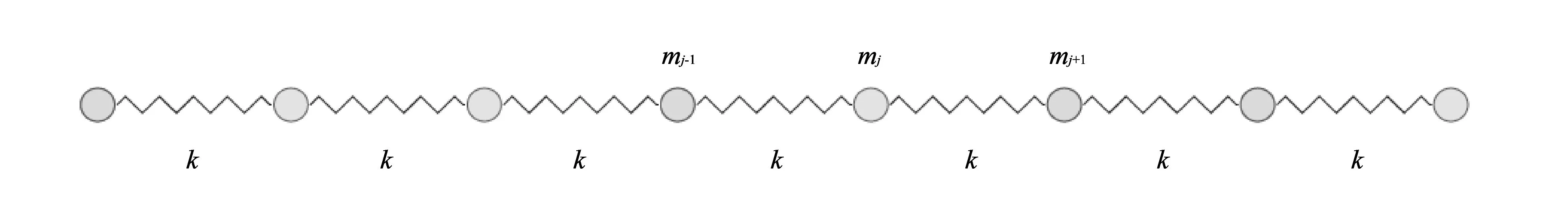
Fig.5 Prouhet-Thue-Morse chain

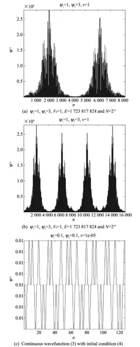
Fig.6 Typical fractal wavefunctions

There is a special case in Eq.(23) model when the unusual continuous wavefunction appears. The main condition is if this case isψ1=ψ2. For example if we set the initial condition as

(24)

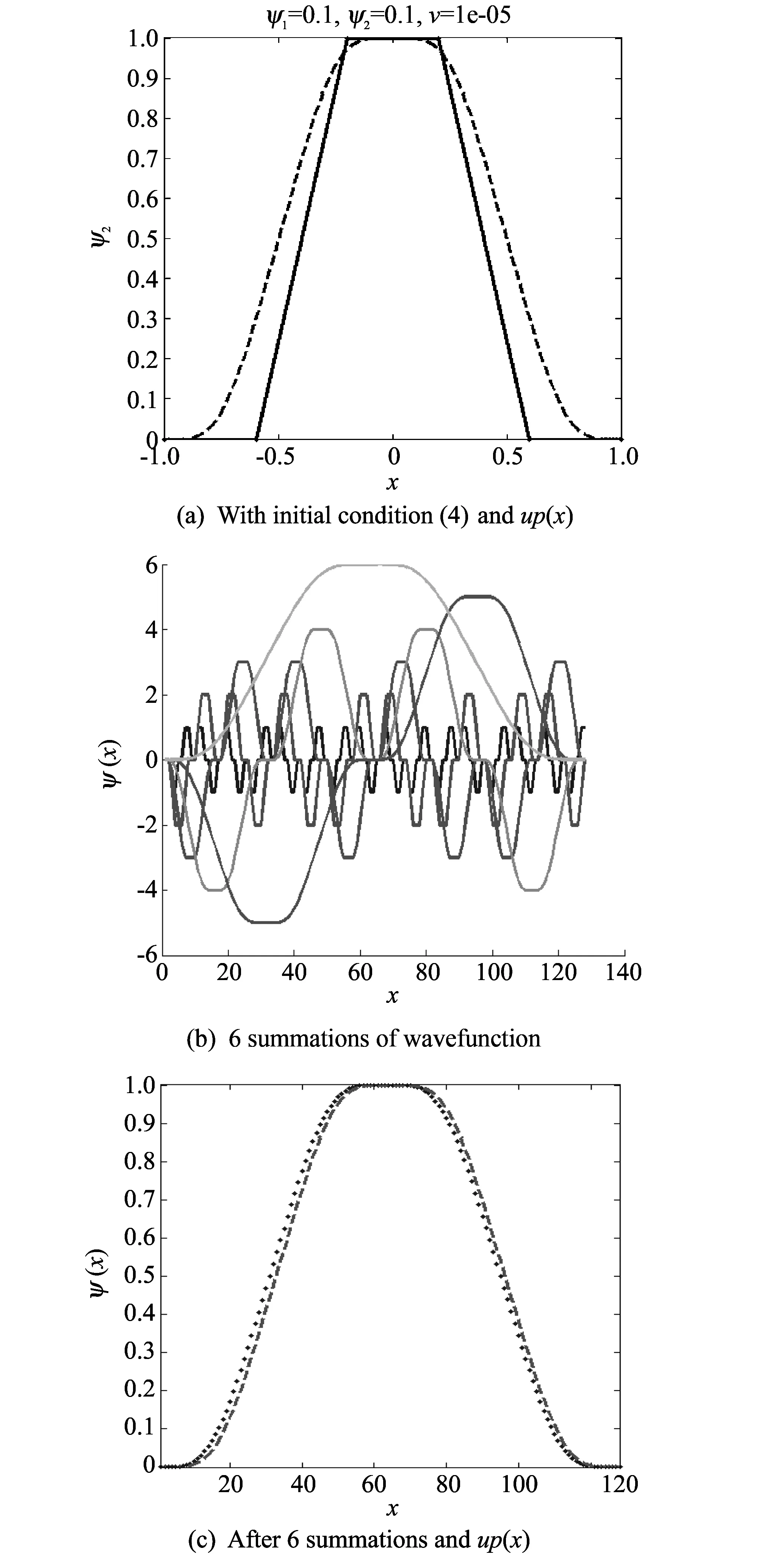
Fig.7 Continuous wavefunctions “hump”

We will obtain the continuous wavefunction as shown in Fig.7(c). Consider the absolute of the normalized vector ψ=ψ-mean(ψ)withthenormalizedψandassumethatthepitsandhumpsarehigh.Infacttheirheightsareslightlydifferent.Sothemeanofthevectorψisclosetozerobutnotzero.Itwillincreaseandsuchkindofstructurewillbeunstableonintegration.InFig.8(a)thecomparisonbetweenthefinitesolutionofEq.(1) up(x) (reddash)andtheabsolutenormalizedhumpofthenormalizedvectorψ≡ψ-mean(ψ) (bluesolid)ispresented.Weperform6summationsofthewavefunctionasinHilberg’salgorithm.WenormalizeeachofthecontinuousfunctiontothemaximumofthemagnitudeshowingthenumberofiterationinFig.8(b).Thenwecompareup(x) (Fig.4(c),reddash)andtheresultinghumpofthe6summationsofthenormalizedvectorψ≡ψ-mean(ψ) (bluedotted,goldlineinFig.8(b)).

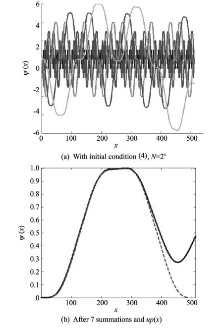
Fig.8 Summations of the wavefunction (3)

Let’sconsiderfour-timesmoreatomsinthePTMchainN=29.Considerthefirst7iterationsofsummationofthewavefunctionasEq.(23)withtheinitialconditionEq.(24),here,wecanseetheunstabletrendontherightpart.

ThegeneralquestionishowwecanobtainEq.(21)fromthewavefunctionEq.(23)withtheinitialconditionEq.(24).So,thereisoneabstractmathematicwaywhichwasintroducedbyJFabius[16].

Supposethatwehavethestablecontinuouswavefunction(i.e.theintegralofthiswavefunctionequalstozero)aftertheiteratedsummations.Forexample,ifwedothesummationNtimes,wecanobtain(undersomeconditions)thesituationwhentheform(orpattern)ofthecontinuousfunctionwiththeN-thiterationwillbedifferentfromtheonewiththeN-1th(orN+1th)iterationonlythescalefactorlikeinFig.7(a) (goldsolidwiththe6thiterationandmagentasolidwiththe5thiteration).

Ifwehavesuchthesituation,wecanapplytheJfabiusformalism.Let’sdefineF(x)as

(25)

Then,defineanotherfunctionf(x)whichisincoincidencewithF(x)on[0,1]andsatisfiestherelations

(26)

Eq.(26)canbetransformedeasilyas

(27)

wherenkisaPTMsequence.Notethatwhilef(x)iscontinuousandvanishesonlyatthenonnegativeevenintegers,itshouldsatisfythefollowingfunctionalintegralequation,

(28)

ByinductionifEq.(27)holdsforall[0,2n]andn≥1,weobtainforx∈(2n,2n+1]

(29)

anditimpliesfromEq.(26)that

(30)

Eq.(29)meansthatitsatisfiesstabilityrequirement,whichissufficient.ItfollowsfromEq.(28)thatf(x)isdifferentiableandcontinuousandsatisfiesthefunctionaldifferentialequation

(31)

forallx∈[0,+∞)andhencef(x)isinfinitelydifferentiablewithn-thderivative,

(32)

forallx∈[0,+∞), n=1,2,….Thereisawell-knownfactfromtheatomicfunctionstheorythatEq.(31)hastheinfinitedifferentialsolutionwhichisaseriesbyup(x)withthePTMcoefficients

(33)

InthepresentinvestigationwehaveconsideredonesimplemodelPTMchainandanativesuggestionhowEq.(1)arisesinsuchkindofmodels.Weusethesummationtechniquewhichplaysakeyroleinoursimpleanalysistosatisfythestabilitycondition.Afterwards,weusetheJ.FabiusformalismtoderivethefunctionalEq.(31)relatedtoEq.(10).

5 Conclusion

In this review we describe briefly recent progress in application of the PTM discrete sequence in different fields such as radar waveform constructions, interferometer measurements, hydrocarbon exploration, and Doppler compensation, etc. We have also defined and considered a family of infinitely differential functions so-called atomic functions which are strongly connected with the PTM sequence in many different senses. On the basis of such a connection a fast iterative algorithm is introduced to solve the accordingly functional-differential equations both single and multi- scaled. We have also presented an investigation of a simple model of the Prouhet-Thue-Morse chain and a native suggestion how could arise in such kind of models which can be a start of a naive physical theory of such kind of functional-differential equations of delay type with scaling.

[1] Nguen H D. A new proof of the Prouhet-Tarry-Escott problem. 2014-11-22[2015-02-17]. http:∥arxiv.org/abs/1411.6168.

[2] Allouche J-P, Shallit J. Automatic sequences: theory, applications, generalizations. London: Cambridge University Press, 2003.

[3] Nguyen H D, Coxson G E. Doppler tolerance, complementary code sets, and the generalized thue-morse sequence, 2014-10-11[2015-02-17]. http:∥arxiv.org/abs/1406.2076.

[4] Hilberg W. Korrelationsermittlung durch stapeln von impulsen: German Patent 198 18 694 A 1, 1999.

[5] Cooklev T. Device and method for compensating or creating doppler effect using digital signal processing: US Patent 6633617 B1, 2003.

[6] Mangum J G. User’s manual for the NRAO 12 meter millimeter-wave telescope. Kitt Peak, Arizona, 2000.

[7] Korotkikh V, Korotkikh G, Bond D. On optimality condition of complex systems: computational evidence, 2005[2015-02-17]. http:∥arxiv.org/abs/cs/0504092.

[8] Rouan D. Ultra deep nulling interferometry using fractal interferometers. Comptes Rendus Physique, 2007, 8(3/4): 415-425.

[9] Chi Y, Pezeshki A, Calderbank R, et al.. Range sidelobe suppression in a desired Doppler interval. In: Proceedings of IEEE International Waveform Diversity and Design Conference, Kissimmee, FL, USA, 2009: 8-13.

[10] Holten T, Flekk y E G, Singer B, et al. Vertical source, vertical receiver, electromagnetic technique for offshore hydrocarbon exploration. First break, 2009, 27(5): 89-93. http:∥www.petromarker.com/wp-content/uploads/2013/06/first-break-may-2009.pdf.

[11] Kravchenko V F, Rvachev V L. Boolean algebra, atomic fucntions, and wavelets in physcial applications. Fizmatlit, Moscow, 2006.

[12] Kravchenko V F. Application of atomic functions theory, WA-systems and R-functions in information technologies. In: Proceedings of International Scientific Seminar "Actual Problems of Mathematical Physics", Moscow State University, Moscow, 2014: 28-33.

[13] Kravchenko V F, Perez-Meana H M, Ponomaryov V I. Adaptive digital processing of multidimensional signals with applications, Fizmatlit, Moscow, 2008.

[14] Zelkin E G, Kravchenko V F, Gusevskii V I. Constructive methods of approximation in theory of antennas. Moscow: Sains-Press, 2005.

[15] Konovalov Y Y. Iterative algorithms for numerical solution of differential equations with linearly transformed argument. International Journal of Electromagnetic Waves and Electronic Systems, 2011, 16(9): 49-57.

[16] Hilberg W, Kravchenko V F, Kravchenko O V, et al. Atomic functions and generalized Thue-Morse sequence in digital signal and image processing. In: Proceedings of 2013 International Kharkov Symposium on Physics and Engineering of Microwaves, Millimeter and Submillimeter Waves, 2013: 66-71.

[17] Konovalov Y Y, Kravchenko V F. Weight functions based on the convolutions of atomic functions. In: Proceedings of the International Conference on Days on Diffraction, 2013: 78-82.

[18] Kravchenko O, A continuous analog of the 1D Thue-Morse sequence, [2015-02-17]. http:∥demonstrations.wolfram.com/A Continuous Analog Of The 1 D Thue Morse Sequence/

[19] Kravchenko O. Polynomial atomic functions for Fourier analysis, 2014[2015-02-17]. http:∥demonstrations.wolfram.com/Polynomial Atomic Functions For Fourier Analysis/

[20] Kravchenko V F, Lutsenko V I, Lutsenko I V. Backscaterring by sea of centimeter and millimeter waves at small grazing angle. Journal of Measurement Science and Instrumentation, 2014, 5(2): 36-43.

[21] Kravchenko V F, Lutsenko V I, Lutsenko I V, et al. Description and analysis of non-stationary signals by nested semi-Markov processes. Journal of Measurement Science and Instrumentation, 2014, 5(3): 25-32.

[22] Volosyuk V K, Kravchenko V F, Kutuza B G, et al. Statistical theory of ultrawideband radiometric devices and systems. Physical Bases of Instrumentation., 2014, 3(3): 5-66.

[23] Kravchenko V F, Churikov D V. Kravchenko atomic transforms in digital signal processing. Journal of Measurement Science and Instrumentation, 2012, 3(3): 228-234.

[24] Kravchenko V F, Churikov D V. Kravchenko probability weight functions in problems of radar signals correlation processing. Journal of Measurement Science and Instrumentation, 2013, 4(3): 231-237.

[25] Volosyuk V K, Kravchenko V F, Pavlikov V V, et al. Statistical synthesis of radiometric imaging formation in scanning radiometers with signal weight processing by Kravchenko windows. Doklady Physics, 2014, 59(5): 219-222.

[26] Volosyuk V K, Gulyaev Y V, Kravchenko V F, et al. Modern methods for optimal spatio-temporal signal processing in active, passive, and combined active-passive radio-engineering systems (Review). Journal of Communications Technology and Electronics, 2014, 59(2): 97-118.

[27] Kravchenko V F, Kravchenko O V, Pustovoit V I, et al. Application of the families atomic functions, WA-systems and R-functions in modern problems of radiophysics. Part I. Journal of Communications Technology and Electronics, 2014, 59(10): 949-978.

[28] Kravchenko V F, Kravchenko O V, Lutsenko V I, et al. Restoration of environment information parameters with using of atomic and WA-systems of functions. Review. Part I. Application of the theory of semi-markov fields and finite functions for the description of non-stationary processes. Physical Bases of Instrumentation, 2014, 3(2): 3-18.

Prouhet-Thue-Morse序列和原子函数在物理和技术中的应用

Victor F Kravchenko1,2, Oleg V Kravchenko1,2,3, Yaroslav Y Konovalov2

(1. Kotelnikov Institute of Radio-engineering and Electronics, Russian Academy of Sciences, Moscow 125009, Russia;2. Bauman Moscow State Technical University, Moscow 105005, Russia;3. Scientific and Technological Center of Unique Instrumentation, Moscow 117342, Russia)

本文系统地阐述了信号与图像处理中与原子函数理论和Prouhet-Thue-Morse序列相关的大量研究成果。

原子函数； Prouhet-Thue-Morse序列； 数字信号处理； 图像处理

Victor F Kravchenko, Oleg V Kravchenko, Yaroslav Y Konovalov. Prouhet-Thue-Morse sequence and atomic functions in applications of physics and techniques. Journal of Measurement Science and Instrumentation, 2015, 6(2)： 128-141.

10.3969/j.issn.1674-8042.2015.02.005

Foundation items： Russian Foundation for Basic Research (No.130212065)

Victor F Kravchenko (kvf-ok@mail.ru)

1674-8042(2015)02-0128-14 doi： 10.3969/j.issn.1674-8042.2015.02.005

Received date： 2015-03-17

CLD number： TN911.7 Document code： A