Analysis of heat pulse signals determination for sediment-water interface fluxes
2014-09-06ZhuTengyiRajendraPrasadSinghFuDafang
Zhu Tengyi Rajendra Prasad Singh Fu Dafang
(School of Civil Engineering, Southeast University, Nanjing 210096, China)
Analysis of heat pulse signals determination for sediment-water interface fluxes
Zhu Tengyi Rajendra Prasad Singh Fu Dafang
(School of Civil Engineering, Southeast University, Nanjing 210096, China)
The heat pulse signal is analyzed in a new way with the goals of clarifying the relationships between the variables in the heat transfer problem and simplifying the procedure for calculating sediment-water interface fluxesJ. Only three parametersx0,λand (pc)lare needed to calculateJby the heat pulse data for this analysis method. The results show that there is a curvilinear relationship between the peak temperature arrival time and sediment-water interface fluxes; and there exists a simple linear relationship between sediment-water interface fluxes and the natural log of the ratio of the temperature increase downstream from the line heat source to the temperature increase upstream from the heat source. The simplicity of this relationship makes the heat pulse sensors an attractive option for measuring soil water fluxes.
sediment-water interface flux; seepage meter; heat pulse; peak arrival time
Direct measurements of water flux across the sediment-water interface can be realized by seepage meters[1-4]. Many environmental scientists are interested in understanding the magnitude and direction of sediment-water interface fluxJat a particular location. This interest arises from the major role ofJin processes such as infiltration, runoff and subsurface chemical transport.Jcan be varied widely in time and space depending on the sediment and environmental conditions. This variability makes the modeling ofJdifficult. In some cases, measuringJdirectly would be a more attractive option than modelingJ. However, only a few practical techniques are available for the measuring ofJin in-situ conditions.
Byrne et al.[5-6]introduced the idea of using heat as a tracer to measureJ. They measured distortion of the steady state thermal field around point and heat sources. Based on the work of Byrne et al.[5-6]and Melville et al.[7], an improved heat pulse technique was developed by Ren et al.[8]to measureJ. The probe used by Ren et al.[8]consisted of three stainless steel needles embedded in a waterproof epoxy body. The center needle contained a resistance heater, and the outer two needles contained thermocouples. This experimental setup is shown in Fig.1. Heat transfer away from the central needle occurred via conduction and convection. The resulting temperature increase at the thermocouples in the two outer needles was measured and recorded by an external datalogger. The convection of heat by the flowing water resulted in a larger temperature increase downstream from the heat source than upstream from the heat source.Tu,TdandHare the upstream sensor, the downstream sensor and the heater, respectively.
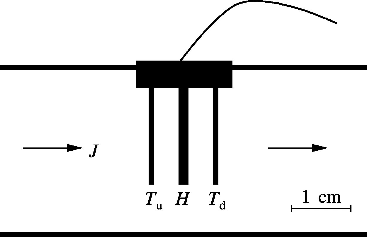
Fig.1 Conceptual drawing of the flow sensor
Ren et al.[8-9]developed an analytical solution for the appropriate heat transfer equation, and explained that this solution could be used to calculateJfrom the difference between the measured temperature increasing at the downstream and upstream needles if the thermal properties of the soil or sediment are known. The main disadvantage of this solution is that it contains an integral that requires the numerical integration. Kluitenberg and Warrick[10]improved the evaluation procedure by converting the equations into the well function for leaky aquifers and by using an infinite series to approximate the well function. Although the improved method eliminates the need for numerical integration, it is still inconvenient to analyze the relationships among variables and to estimateJbecause the infinite series is quite complicated.
Hence, in this paper we analyzed the heat pulse signal in a new way with the goals of clarifying the relationships between the variables in this heat transfer problem and simplifying the procedure for calculatingJfrom heat pulse measurements.
1 Theory
1.1 General solution for heat transfer equation
The theory of heat flow has been a subject of investigation for centuries. Numerous papers and books have been written on this subject. Probably the most comprehensive book on the subject within the last century was “Conduction of heat in solids” by Carslaw and Jaeger[11]. When the developed theories are applied to physical problem, it is often necessary to approximate either the initial or boundary conditions. For a simple solution that can describe the thermograph, one would either want an instantaneous pulse of heat, a step of heat, or a square wave pulse. None of the normally assumed initial conditions are reasonable explanation of the heat input produced by the heater. As a result, the shape of the thermograph observed in the physical system is inconsistent with the shape produced by the common mathematical developments. To overcome this problem, Taniguchi et al.[12]proposed using the time when the peak temperature is detected at the thermistors to determine the velocity of the heat. They took the derivative of an analytical solution with ideal boundary conditions. The peak temperature occurs when the derivative equals zero. Their development yields the following equation whentmax> 0 andU>0:
(1)
whereUis the velocity;tmaxis the peak temperature arrival time measured by the thermistor at distancexfrom the heat source; andκis the thermal conductivity of water divided by the specific heat and density.
The water velocity is proportional but not equal to the thermal velocity. If one can assume that there is no thermal gradient in the radial direction (instantaneous heat transfer in the radial direction) and there is no heat loss from the pipe, then the thermal velocity will be slower and directionally proportional to the water velocity. The technique proposed by Taniguchi and Fukuo[12]is suitable for measuring the higher flow rates when the advective process dominates. It uses the difference in peak arrival times between thermistors to estimate flow rates.
Ren et al.[8]proposed a solution using heat transfer equation analysis to determine the heat pulse:
(2)
whereTis the temperature increase, ℃;tis the time,s;αis the thermal diffusivity of water,m2/s-1; andxandyare the space coordinates (distance between the thermistor and the heat source); andVis the velocity, m/s.
Ren et al.[8]presented a solution for Eq.(2) corresponding to a heat pulse produced by an infinite line source in an infinite, homogenous, porous media through which water is flowing uniformly,
0 (3) t>t0 (4) whereqis the heating power,W/m;t0is the heat pulse duration, s;Vis the heat pulse velocity;λ=αρcis the thermal conductivity,W/(m·℃)-1;s=t-t′. This solution is based on the assumption that the conductive heat transfer dominates over the convective heat transfer. The temperature increase at a distanceχddirectly downstream from the line source is (5) (6) The temperature increase at a distanceχddirectly upstream from the line source is (7) (8) The flux meter typical temperature increase vs. time curves generated using Eqs.(5) to (8) is shown in Fig.2. Fig.2 Typical temperature increase vs. time curves (V=5×10⁻⁵m/s,α=1.4×10-7m2/s,λ=0.58 W/(m·K)-1,χ0=0.005 m, q=40 W/m for heating of 6 s, q=20 W/m for heating of 3 s) 1.2 Difference of downstream and upstream temper-ature increases Ren’s method is not exactly suitable for determining seepage flux meter due to the large heat losses transferred to the air and water. It is also hard to determine how much energy will be lost in the system. But it is useful to analyze temperature distribution, so we focus on the analysis of dimensionless temperature difference (DTD). This solution is as follows: (9) Eq.(9) indicates that the dimensionless temperature difference is a function ofV,t0,qand the thermal properties of the water. Fig.3 shows the heat pulse signal converted to the DTD. The maximum value of the DTD (MDTD) is given by MDTD= (10) wheretmis the time at which DTD reaches a maximum. By evaluating Eq.(10) forVon the order of 10-5m/s, we found a close linear relationship betweenVand MDTD. Graphical evaluation of Eq.(10) reveals a close unique relationship between MDTD andV(see Fig.4). This result is in consistent with the results of Ren et al[8]. This relationship suggests that measurement of MDTD can provide a useful means of estimatingV. Fig.3 Heat pulse signal converted to DTD 1.3 Ratio of downstream and upstream temperature increases By dividing Eq.(6) with Eq.(8) for a heating period, we can get the ratio of downstream and upstream temperature increases whenxd=xu=x0. (11) Fig.4 Relationship between MDTD and V Eq.(11) demonstrates that whenxd=xu=x0, the ratio of the downstream temperature increase to the upstream temperature increase (Td/Tu) is independent of time[13]. Whenxd=xu=x0,Td/Tuis only a function ofx0,Vandα, unlike MDTD, independent oft0,λandq. Fig.5 shows the heat pulse signal converted toTd/Tuand reveals that there is no significant difference between 3 and 6 s heating condition. Fig.5 Heat pulse signal converted to Td/Tu The main objective of this new analysis is to clarify the relationships between the key variable in the heat pulse technique for measuringJ. Three interesting relationships were revealed by this new analysis and some implications of the relationships were also studied. First, Eq.(11) reveals thatTd/Tuis a function of a single dimensionless number,Vχ0/α. Fig.4 shows MDTD and ln(Td/Tu) as functions ofVχ0/α. The slope of the MDTD vs.Vχ0/αrelationship depends on the values ofχ0,α,t0,qandλ, but the slope of ln(Td/Tu) vs.Vχ0/αshould always be equal to the one as long as conduction is the dominant mechanism of the heat transfer. The second interesting fact about the heat pulse technique revealed by this new mathematical analysis is that wheneverxd=xu, the maximum temperature increases at the upstream and downstream positions occur simultaneously regardless of the magnitude ofV. The heat pulse signal travels upstream just as rapidly as it does downstream. The magnitude of the signal is decreased in the upstream direction. The third noteworthy finding of this mathematical analysis is a new insight into the relationship between MDTD andJ. Ren et al.[8]found a close linear relationship between MDTD andV, but they were unable to explicitly state the form of the relationship due to the complexity of their solution equation (Eq.(10)). To consider the relationship betweenJandTd/Tu, if we combine Eq.(11) andV=J(pc)l/pc(whereρcis the volumetric heat capacity of the multiphase system,J/(m3·C)-1; (pc)lis the volumetric heat capacity of the liquid), we can obtain the following equation: (12) The explicit form of Eq.(12) can make it very useful for designing an implement calibration procedure. In this case, only three parametersx0,λand (pc)lare required when we use Eq.(12) to calculateJfrom heat pulse data compared with the procedures of Ren et al[8]. Another objective of this study is to simplify the procedure for calculatingJfrom the heat pulse in cases where the soil thermal properties are known. In this case, to calculateJfrom heat pulse measurements using the Ren’s equations requires a numerical integration routine coupled with a nonlinear regression routine. With these two routines one can obtainJ. These are all simple, explicit equations that can be easily evaluated using a simple calculator or a data logger.λis the soil thermal property used to calculateJ(Eq.(12)). In the case, the soil thermal properties are not knownapriori, and it is not clear whether it is possible to calculateJusing Ren’s equations (Eq.(2)). However, the results of our analyses show that we can obtain some information from the heat pulse data even withoutaprioriknowledge of the soil thermal properties.Vcan be calculated from Eq.(11) and Eq.(12). OnceVis known, only an estimate ofρcis needed to calculateJ. Using Eq.(12), only three parametersx0,λand (pc)lare needed to calculate the water flux densityJfrom heat pulse data. Ren’s method has some disadvantages. The first is that the calculation requires numerical integration, which is not trivial and may induce some error. The second disadvantage is that they used only a single data point, the MDTD. The measurement accuracy of that single point will directly affect the calculatedJ. The new analysis presented in this paper enables an average value ofTd/Tuover an appropriate time interval to be used with Eq.(11) to calculateV, which can be converted toJ. This averaging can reduce the influence of measurement error in a single data point. The previous methods do not provide any method to calculateVifαis unknown; however, this new analysis still needs to be improved upon. [1]Lien B K. Development and demonstration of a bidirectional advective flux meter for sediment-water interface[R]. Cincinnati, OH, USA: National Risk Management Research Laboratory, Office of Research and Development, US Environmental Protection Agency,2006:12-40. [2]Smith A J, Herne D E, Turner J V. Wave effects on submarine groundwater seepage measurement[J].AdvancesinWaterResources, 2009, 32(6): 820-833. [3]Mwashote B, Burnett W, Chanton J, et al. Calibration and use of continuous heat-type automated seepage meters for submarine groundwater discharge measurements[J].Estuarine,CoastalandShelfScience, 2010, 87(1): 1-10. [4]Swarzenski P W, Izbicki J A. Coastal groundwater dynamics off Santa Barbara, California: combining geochemical tracers, electromagnetic seepmeters, and electrical resistivity[J].Estuarine,CoastalandShelfScience, 2009, 83(1): 77-89. [5]Byrne G, Drummond J, Rose C. A sensor for water flux in soil.“Point source” instrument[J].WaterResourcesResearch, 1967, 3(4): 1073-1078. [6]Byrne G, Drummond J, Rose C. A sensor for water flux in soil. 2. “Line source” instrument[J].WaterResourcesResearch, 1968, 4(3): 607-611. [7]Melville J G, Molz F J, Güven O. Laboratory investigation and analysis of a ground-water flowmeter[J].GroundWater, 1985, 23(4): 486-495. [8]Ren T, Kluitenberg G, Horton R. Determining soil water flux and pore water velocity by a heat pulse technique[J].SoilScienceSocietyofAmericaJournal, 2000, 64(2): 552-560. [9]Wang Q, Ochsner T E, Horton R. Mathematical analysis of heat pulse signals for soil water flux determination[J].WaterResourcesResearch, 2002, 38(6): 27-1-27-7. [10]Kluitenberg G, Warrick A. Improved evaluation procedure for heat-pulse soil water flux density method[J].SoilScienceSocietyofAmericaJournal, 2001, 65(2): 320-323. [11]Carslaw H S, Jaeger J C.Conductionofheatinsolids[M]. 2nd ed. Oxford: Clarendon Press, 1959. [12]Taniguchi M, Fukuo Y. Continuous measurements of groundwater seepage using an automatic seepage meter[J].GroundWater, 1993, 31(4): 675-679. [13]Kluitenberg G, Ochsner T, Horton R. Improved analysis of heat pulse signals for soil water flux determination[J].SoilScienceSocietyofAmericaJournal, 2007, 71(1): 53-55. 沉积物-水界面通量测定中热脉冲信号分析 朱腾义 Rajendra Prasad Singh 傅大放 (东南大学土木工程学院, 南京 210096) 分析了热脉冲传感器脉冲信号与沉积物-水界面通量之间的传热问题,并通过优化程序,提出了用热脉冲测定计算界面通量J的新方法.此分析方法只需3个实验参数,即x0,λ和(pc)l就可利用热脉冲测定数据计算出沉积物-水界面通量J.数据分析结果表明:热脉冲顶点温度到达时间与水流速度呈曲线关系;沉积物-水界面通量和热源上下游温升比值的自然对数之间存在一种简单的线性关系.这种简单的线性关系,有利于热脉冲型传感器在土壤-水界面通量测定中的广泛应用. 沉积物-水界面通量; 渗流仪; 热脉冲; 顶点温度到达时间 X830.3 The Priority Academic Program Development of Jiangsu Higher Education Institutions. :Zhu Tengyi, Rajendra Prasad Singh, Fu Dafang.Analysis of heat pulse signals determination for sediment-water interface fluxes[J].Journal of Southeast University (English Edition),2014,30(2):192-196. 10.3969/j.issn.1003-7985.2014.02.010 10.3969/j.issn.1003-7985.2014.02.010 Received 2013-10-18. Biographies:Zhu Tengyi (1984—), male, graduate; Fu Dafang (corresponding author), male, doctor, professor, fdf@seu.edu.cn.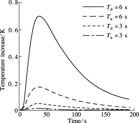


2 Discussion
3 Conclusion
猜你喜欢
杂志排行

Journal of Southeast University(English Edition)的其它文章
- Prediction on effectiveness of road sweepingfor highway runoff pollution control
- A preliminary sustainability assessment of innovativerainwater harvesting for residential properties in the UK
- Approach to estimating non-point pollutant load removal rates based on water environmental capacity: a case study in Shenzhen
- Potential contributions to Beijing’s water supply from reuse of storm- and greywater
- Characteristics of Hg pollution in urban stormwater runoff in Nanjing city, China
- Rainwater harvesting in the challenge of droughts and climate change in semi-arid Brazil