A Real-time Updated Model Predictive Control Strategy for Batch Processes Based on State Estimation*

YANG Guojun (杨国军), LI Xiuxi (李秀喜) and QIAN Yu (钱 宇)

School of Chemical Engineering, South China University of Technology, Guangzhou 510640, China

A Real-time Updated Model Predictive Control Strategy for Batch Processes Based on State Estimation*

YANG Guojun (杨国军), LI Xiuxi (李秀喜) and QIAN Yu (钱 宇)**

School of Chemical Engineering, South China University of Technology, Guangzhou 510640, China

Nonlinear model predictive control (NMPC) is an appealing control technique for improving the performance of batch processes, but its implementation in industry is not always possible due to its heavy on-line computation. To facilitate the implementation of NMPC in batch processes, we propose a real-time updated model predictive control method based on state estimation. The method includes two strategies: a multiple model building strategy and a real-time model updated strategy. The multiple model building strategy is to produce a series of simplified models to reduce the on-line computational complexity of NMPC. The real-time model updated strategy is to update the simplified models to keep the accuracy of the models describing dynamic process behavior. The method is validated with a typical batch reactor. Simulation studies show that the new method is efficient and robust with respect to model mismatch and changes in process parameters.

batch process, exothermic batch reactor, nonlinear model predictive control, state estimation, real-time model update

1 INTRODUCTION

Batch processes are widely applied to manufacture a large quantity of value-added products such as pharmaceuticals, biological products, polymers and electronic chemicals. The application of advanced process control techniques in these processes can improve process performance and product quality. However, most batch processes exhibit highly nonlinear and time-varying behavior, making the control of such processes complex and challenging. In addition, an important control objective for batch processes is to realize perfect tracking of set-point profile, and thereby guarantee good product quality. To address these issues, model predictive control (MPC) has been applied to batch processes [1-4] and is widely recognized as an efficient control technique for desired performance of batch processes.

The ability to handle nonlinearities in process dynamics and economical objective functions makes nonlinear model predictive control (NMPC) especially useful for batch process control. A number of NMPC studies dealt with the control of polymerization reactors [5], batch distillation [6], batch crystallization [7], and so on [8]. Gao et al. [9] proposed an online iterative learning model predictive control method for controlling a multi-phase batch process. Kansha and Chiu developed an adaptive generalized predictive control strategy based on the just-in-time learning (JITL) technique for nonlinear process control [10]. Escano et al. developed a strategy by integrating neuro-fuzzy model with NMPC and implemented it in a pilot plant successfully [11]. However, the implementation of NMPC based on the first principle process model in large-scale or industrial applications is not always possible. One of the reasons is the computational complexity of the NMPC. This leads to two problems: (1) the computational time for solving NMPC problems exceeding real-time requirements; (2) insufficient accuracy or stability of the controller.

There are many ways to reduce the computational complexity of NMPC [12]. One way is to develop efficient and reliable solution methods for NMPC problems. A series of high-performance solution methods [13-16] for NMPC problems have been developed to make NMPC a viable control technique [17, 18], but the computation is still too intensive to use conventional process control computers for on-line implementation. An obvious difficulty is that the optimization problem is nonlinear and has a large number of decision variables. Another way is to use multiple reduced models [19] or empirical models [20-22] instead of the first principle process model, reducing the computation of models, which is a popular way for enhancing the applicability of NMPC, especially in the present situation with limited computational power available in industries. Kuure-Kinsey and Bequette have developed a multiple model predictive control strategy for controlling process systems with disturbances [23, 24]. By incorporating four different disturbance models to a nominal linear model representing the expected system operating condition, the strategy can estimate and reject different types of unmeasured disturbances. Peterson et al. proposed a nonlinear dynamic matrix control algorithm, which can real-time update the linear model subject to the difference between linear and nonlinear model responses, and applied it to a semi-batch polymerization reactorsuccessfully [25]. Dougherty and Cooper proposed a practical multiple model adaptive strategy for multivariable MPC [26]. Wang et al. proposed a multiple model approach for robust control of non-linear processes [27]. Bonis et al. integrated successive local linearization with model reduction technique to reduce the computational cost of MPC for nonlinear distributed parameter systems [28].

For the multiple model based approach, determination of optimal model switching policy is as crucial as the accuracy of the models. To automatically select the model used in NMPC, Dones et al. have proposed a self-adaptive approach for NMPC to adjust the dimension of the model according to current process conditions and control objectives [29]. This approach can adapt the model in the MPC algorithm to current operating conditions of the plant. However, the algorithm is mainly focused on special processes, in which a set of simplified models is obtained by reducing the number of dynamic equations in the full model. For most of other batch processes whose simplified models cannot be obtained in this way, this algorithm is not always feasible. Kansha and Chiu have proposed a JITL based NMPC method to update the data-based model used in NMPC on line [10]. Owing to its high efficiency, the method has been successfully applied in many batch processes [30]. Nevertheless, the feasibility and performance of the method largely depends on the reliability of the data-based modeling technology, which makes the method more suitable for the processes with lots of historical data and similar operation conditions for each cycle.

In this work, we propose a real-time updated model predictive control (RTUMPC) strategy for realizing perfect tracking along the optimal trajectory for the operation of batch process [31]. It combines a multiple model building technique with a real-time model updated strategy to improve the computational efficiency of NMPC and keep good performance of NMPC for process control. The multiple model building technique is based on model linearization, producing a series of simplified models with different complexity by locally linearizing the nonlinear relationship among the variables in the control system. The real-time model updated strategy is used for keeping the accuracy of the simplified models to describe the actual system by updating the models real time according to current process conditions. The real-time update of the simplified models is implemented based on state estimation, so it is important to select an efficient and reliable state estimator for the controlled system. Successful application of the model-based control largely depends on the accuracy of the information about the states of the system provided by the estimator. A series of work has been focused on the development of feasible and reliable nonlinear state estimators [32-34], which have promoted the development of model based control technology.

2 REAL-TIME UPDATED MPC STRATEGY

2.1 NMPC formulation

In NMPC algorithm, a sequence of control moves is computed at each control interval to minimize an objective function, subject to constraints on input and output variables, as well as constraints imposed by nonlinear dynamic model equations. The first input in the optimal sequence is implemented. For the next control intervals, the objective function and model equation constraints are updated on the basis of new measurements and state variable estimates. Then, all these steps are repeated. For the NMPC of batch process, after the optimal set-point trajectory of the process is determined by dynamic optimization method [35], the optimal control problem for realizing perfect tracking along the trajectory can be formulated as

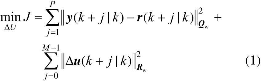
subject to

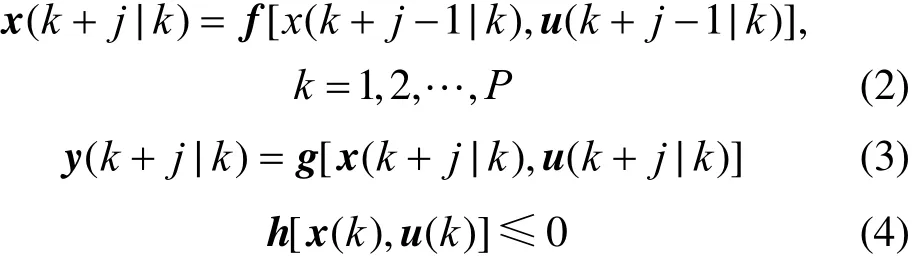
where J is the dynamic performance objective, Qwand Rware the weighting matrixes of appropriate dimensions, P is the prediction horizon, M is the control horizon, and k is the current sampling interval. The state variable vector isis the predicted output vector of the system, and r is the reference signal.is the sequence of future inputs,is the vector function of dynamic equations of the system, g: output,is the vector functions that describe all of the system inequality constraints, which are linear and nonlinear, time-varying or end-time algebraic constraints.

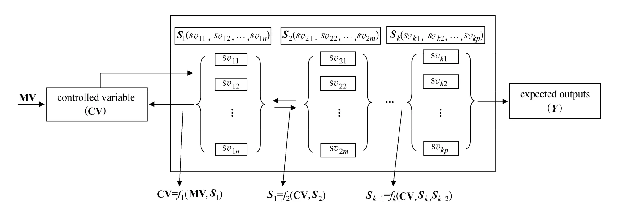
Figure 1 Strategy of decomposing nonlinear process system

NMPC problem is a nonlinear program (NLP) problem, which can be represented by nonlinear objective function equation (1) and nonlinear constraint equations (2)-(4). The solution efficiency of NMPC problem and the accuracy of process model to describe the system behavior are the key factors for successful implementation of NMPC [12]. Thus a large scale complex system can make the control task challenging. In addition, due to their nonlinear and time-varying nature, batch processes are operated in multiple regions under different process conditions with different initial states [5]. These situations force the process model used in NMPC to be updated alongis the vector function of system system trajectory. To meet such requirements, two strategies are introduced here. One is the multiple model building strategy, which simplifies the original system model to a series of simple models based on linearization of the nonlinear functions. The simple models include lots of linear models and nonlinear models with different accuracy for describing the system behavior. Moreover, these simple models show different complexity and provide multiple selections for representing the system in different operating regions, relieving the computational task of NMPC and improving the robustness of system control. The other one is the real-time model updated strategy, which is in charge for updating the simple models as prediction model in NMPC problem. This strategy is based on state estimation of the system to select and update the model used in NMPC according to current states of the system. Integration of the two strategies can improve the on-line solution efficiency of NMPC problem as far as possible while maintaining the performance of NMPC for process control. However, it should be mentioned that the successful application of the proposed strategies subjects to some preconditions: the models used in NMPC are built based on first principles; the state variables of system can be measured or observed, which determine the amount of process state information for model update.

2.2 Strategy for multiple model building

The quality of multiple models has significant effect on the performance of NMPC based on multiple models. Development of efficient and reliable approach for multiple model building plays an important role in enhancing the applicability of NMPC technique. The simplest way to get a series of simple models is to perform linearization based on the system Jacobian in every time interval. This yields successive linearization MPC (SLMPC) [19, 28, 36]. However, it is difficult for a linear model to ensure the accuracy to describe an actual system, especially for a highly nonlinear system, which leads to poor performance of the SLMPC for process control. Therefore, a promising way is to partially linearize the system model to produce a series of simplified models, which can keep some degree of nonlinearity and retain a satisfactory efficiency for problem solution.

For controlling time-invariant batch processes, one of the operation tasks is to realize perfect tracking of desired set-point trajectory in each cycle [37]. Based on the optimal control structure design [38-41], the controlled variables in batch process are always selected from those easy to measure, easy to control by using one of the available manipulated variables, and presenting strong effect on products or performance of plant. The interaction among the manipulated variable (MV), controlled variable (CV), state variables (SV) and process outputs are described in Fig. 1.

According to the interaction among variables, the system dynamics of the batch process can be represented by a number of nonlinear functions, so that it is easy to acquire a series of simplified models by selectively linearizing the functions. Obviously, linearizing different nonlinear functions produces different simplified models with different level of detail of the system dynamics because of different degrees in the nonlinearity of nonlinear functions. In this way, a series of simplified models with different complexity and different accuracy to represent the system can be obtained based on the original system model. With the batch process in the structure as shown in Fig. 1, a series of simplified models can be obtained by selectively linearizing nonlinear functions f1, f2,…, fk. Thesimplified models include model SM(1) obtained by completely linearizing the full system model, model SM(2) by linearizing nonlinear function f1, and the kth simplified model SM(k), as shown in Fig. 2.

Figure 2 Diagram of simplified models of batch process system

In NMPC, complete linear models can be used when the nonlinear system is operated at relatively stable state with small set-point change and disturbances. Partially linearized models can be used when the system characteristics is changed dramatically. The models are selectively used according to a designed strategy, which will be discussed in the next section.

2.3 Strategy for real-time model update

A number of ways [26, 27, 42] based on predefined situation have been introduced to manage the multiple models used in NMPC. To manage the models more automatically, a self-adaptive approach has been proposed by Dones et al. [29], which decides the model used in NMPC based on current process conditions and control objectives. However, model selection only in the approach can not assure the accuracy of model used in NMPC due to the parameter uncertainty and disturbances in the process. Hence, to maintain the accuracy of the simplified models to represent actual system, the models need to be updated according to current states of the system. Before establishing the real-time model updated strategy, it is better to give the simplified models different selection orders (high selection order means high priority to be selected). It should be noted that the selection order may be different in different situations. When the system is operated under a normal condition without disturbances, simpler model has higher selection order since it can save computational time for problem solution, but when the system operation is disturbed, simpler model has lower selection order for its lower accuracy to describe the system.

Three criteria for model update are established in this study. The first one is based on parameter estimation. A parameter estimator is used to estimate the value of uncertain parameters and to calculate the difference between current used valuecurkP and estimated value of parameterestkP . If the percentage variation of the parameter is larger than a certain tolerance εpset by user,

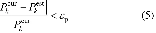
the simplified models will be updated according to current operating condition.

The second criterion is based on the set-point change of controlled variables. In a series of appropriate ranges of set-point change (SC) established for the simplified models, the set-point change that is known in priori will decide which model should be selected to be used to guarantee the performance of NMPC. The third criterion is based on the differences between predicted outputs of the simplified models and actual outputs of the system. Each of the models has a predefined largest limit limoutfor the output difference. If the absolute value of the output difference εoutis larger than limoutfor current model, a more accurate model with larger limit of output difference will be selected to be used in the NMPC at the next time interval.

Figure 3 Flowchart of the real-time model updated strategy for NMPC of batch process based on multiple models

The procedure of real-time model updated strategy is illustrated in Fig. 3. At the beginning, state estimator is used to detect parameter change and decide whether the simplified models should be updated. Then set-point change is detected to judge whether the current used model can deal with the change. If not, another more appropriate model will be selected to beused in the NMPC for the next time interval. If yes, the output differences between simplified models and actual process will be calculated to judge whether current model is appropriate and to decide which model will be more appropriate as the prediction model in NMPC for next time interval. If all of the output performance of the models is acceptable, the simplest model is always the first selection. When the outputs of the actual system deviate much from the predicted outputs, the model with the highest accuracy is always selected.

2.4 Feasibility and performance analysis

The RTUMPC algorithm is an extension of earlier SLMPC technique developed for nonlinear processes [19, 28, 43]. SLMPC is consistent with RTUMPC based on linear model, SM(1) in Fig. 2. SM(1) is the one with the simplest structure and lowest fidelity with respect to the original nonlinear model in the multiple models built in Section 2.2, indicating that the model used in RTUMPC has a higher quality than that used in SLMPC. Consequently, it makes the RTUMPC algorithm more stable and feasible than the SLMPC algorithm for nonlinear process control. In addition, as long as the multiple models used in RTUMPC can maintain a certain level of prediction accuracy to the actual system, the stability of RTUMPC is equivalent to that of standard NMPC, which means that the NMPC stability results presented in literature [12, 44, 45] are also suitable for RTUMPC.

The RTUMPC algorithm takes advantage of multiple model building and real-time model update. On the one side, since the model used in RTUMPC is the reduced model from the original system model, the on-line solution for RTUMPC problem is more efficient than that for normal NMPC problem. On the other side, owing to the real-time model updated strategy, which can make the reduced models keep a high fidelity with respect to the original system model along the computed system trajectory, the RTUMPC algorithm can maintain high performance for process control. Consequently, the RTUMPC approach provides a compromise between control performance and on-line computation, so that the RTUMPC algorithm is more suitable for the on-line implementation in industrial processes than normal NMPC.

The robust performance of the RTUMPC algorithm mainly depends on the performance of state estimator. Although a large number of stable nonlinear observers have been developed [33, 34], the rigorous robustness analysis [46] for the RTUMPC based on state estimation is not a simple work since most of batch processes are dynamic system with no steady state and there are various disturbances, such as model mismatch and change of unmeasured parameters. The robust performance of the RTUMPC algorithm is evaluated by simulation studies in the next section.

3 CASE STUDY: EXOTHERMIC BATCH REACTOR

A reaction system consisting of a batch reactor and a jacket cooling system [47] is shown in Fig. 4. In the reactor, two parallel highly exothermic reactions occur:

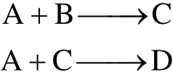
where A and B are the raw materials, C is the desired product, and D is the by-product. The production rates of C and D are R1and R2, respectively, with R1=k1MAMBand R2=k2MAMC, where k1and k2are the rate constants dependent on the reaction temperature through the Arrhenius relation. MA, MB, MCand MDare the number of moles of components. A full description of the reactor system has been given in [47, 48].

3.1 Dynamic model

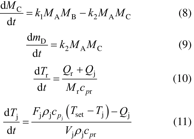
The equations with the first principle system model of the batch process are as follows [48]

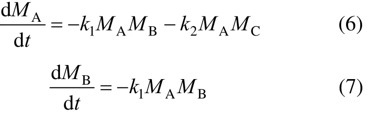
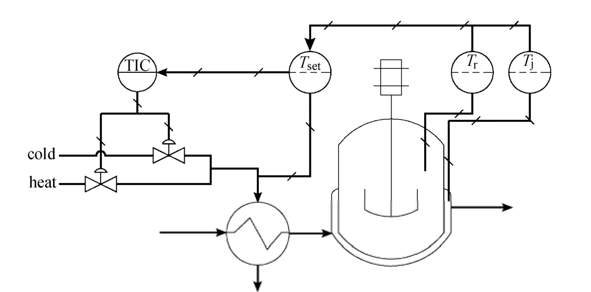
Figure 4 Schematic diagram of batch reactor

with

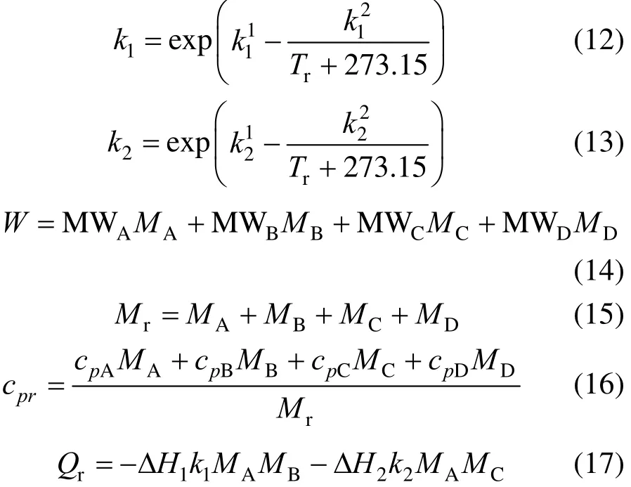
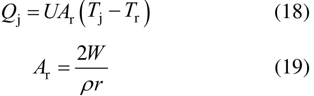
where Tris the reactor temperature, Tjis the jacket temperature, Tsetis the set point value of jacket temperature, W is the mass of reactor contents, Mris the total moles of contents, cpris the heat capacity of contents, Qris the reaction heat, Qjis the heat transferred to the reactor from the jacket, and Aris the heat transfer area of the reactor. The model parameters for the reactor simulation are presented in Table 1, which are from [47, 48].

Initial conditions and strategy for measurements are set as follows. The initial values for MA, MB, MCand MDare 12, 12, 0 and 0 kmol, respectively. The initial value for both Trand Tjis 20 °C. The sample time for temperature measurement is 0.1 min and that for reactant concentrations is 1 min.

3.2 Multiple model building

Figure 5 shows the relationship among the variables in the batch reactor. Controlled variable Trhas significant effect on the production of C and D, manipulated variable Tsetmanipulates the jacket temperature Tjby heat-exchanger, and subsequently, Tjhas a direct effect on Tr. The nonlinear relationship among the manipulated variables, controlled variables and state variables can be expressed by a series of nonlinear functions. Function f1represents the relationship between manipulated variable Tsetand variable Tj. Function f4represents the relationship among controlled variable Tr, state variables Tjand Qr. Function f2represents the relationship between controlled variable Trand rate constants k1and k2. Subsequently, the rate constants affect state variables MA, MB, MC, and MD, represented by function f3.

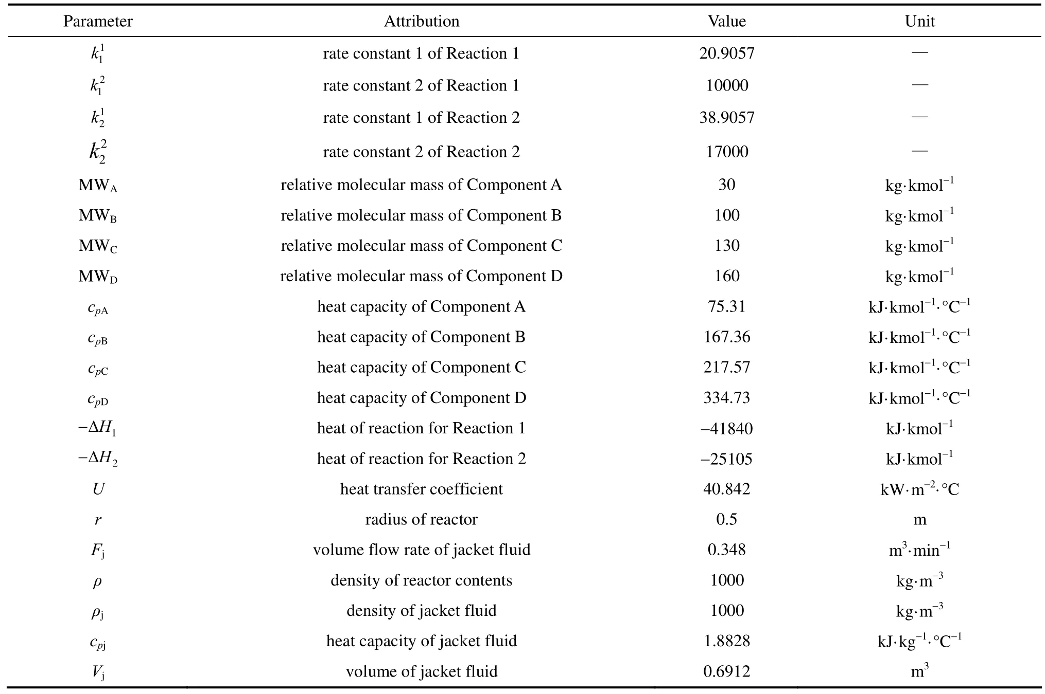
Table 1 Parameters used in the dynamic model of batch reactor

Figure 5 The relationship diagram of variables in the batch reactor

By selectively linearizing the nonlinear relationships, the original system model are reduced to three simplified models. Simplified model 1 (SM1) is based on the linearization of function f3. Simplified model 2 (SM2) is based on the linearization of functions f2and f3. Simplified model 3 (SM3) is a linear model obtained by completely linearizing the original system model. The performance of the simplified models is tested by dynamic simulation, in which two situations are considered: a step change in the manipulated variable and a series of step changes in the manipulated variable. Results are shown in Figs. 6 and 7. Simplified models SM1, SM2 and SM3 describe the system in different levels of accuracy. By comparing their responses with that of original nonlinear system model (NM), it is found that the response difference between SM1 and NM is the smallest, while that between SM3 and NM is the largest. Thus the model with lower degree of linearization has higher accuracy to represent actual system. However, lower degree of model linearization leads to more complex model. For the solution of NMPC problem, more complex model constraint equations need more time to solve the problem.

Figure 6 Response of four different models with a step change (50 °C) in manipulated variable

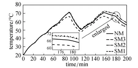
Figure 7 Response of four different models with a series of step changes in manipulated variable

Table 2 shows the computational time for optimization of control problem in NMPC based on the simplified models. The computation based on SM3 costs the shortest CPU time, because it is a linear model and consequent control problem is actually transferred to a linear model predictive control (LMPC) problem, which can be solved with simple quadratic programming (QP). The required CPU time is reduced in the order of NM, SM1 and SM2, because the complexity of the three models is reduced in this order and the time required for solving NLP problem is consequently reduced. In the CPU time test, the LMPC problem is solved with a QP solver, with the NMPC problem converted into an NLP problem by discretizing state and control variables using collocation on finite elements and the NLP problem solved by successive quadratic programming (SQP) method. The CPU time corresponds to an implementation in MATLAB (R2011a) single-threaded code and execution on a workstation based on Intel(R) Core(TM) 2 Duo processors (2.66GHz) and 4 GB of RAM, running a 32-bit distribution of Win7 ultimate.

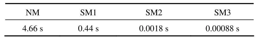
NM SM1 SM2 SM3 4.66 s 0.44 s 0.0018 s 0.00088 s

3.3 Real-time updated model predictive control

The RTUMPC method is used to control the reactor temperature Trto follow an optimal trajectory. The control performance of RTUMPC is compared with that of LMPC, generic model control (GMC) and nonlinear model predictive control based on full dynamic model (standard NMPC). In addition, a series of tests are used to investigate the robustness properties of the RTUMPC. Before the implementation of the algorithm to the batch reactor, the optimal trajectory of the reactor temperature Tris determined and a state estimator is designed for state and parameter estimation.

3.3.1 Optimal profile of reactor temperature

The optimal temperature profile is assumed to be perfectly tracked and determined off-line. The general operating objective for the batch reactor is to maximize the amount of product C,where J is the terminal cost representing the amount of product C at the final time (tf=200 min) of each cycle. The constraints for the objective are Eqs. (6)-(9), (12), and (13).

The objective and constraints compose a dynamic optimization problem. A large number of efficient and reliable solution methods for dynamic optimization problem have been introduced by Biegler [13]. In this study, a simultaneous approach is used to solve the problem, the basic idea of which is to convert the dynamic optimization problem into an NLP problem by approximating state profiles with collocation on finite elements. Then a general SQP method is applied to solve the NLP problem. The results of dynamic optimization with different time intervals are presented in Fig. 8. The amount of product C at the final time increases with the number of intervals, because the approximate optimal profile of reactor temperature with piecewise constant policy is close to actual optimal profile as the number of intervals increases.

Figure 8 Optimal profile of reactor temperature with different intervals

3.3.2 State estimator design

The success of the RTUMPC largely depends on the ability to measure, estimate or predict state variables, outputs and parameters of the process at any given period. There are many advanced nonlinear state estimators [33, 49] for nonlinear state estimation. A commonly used estimator, extended Kalman filter (EKF) estimator, is used in this study for its success in the state estimation of batch reactor [47, 48].

We consider the dynamic model for state and parameter estimation as follows

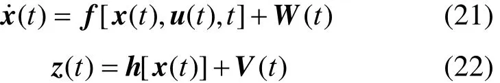
where f is a vector of system function, h is a vector of measurement function, W is a zero mean Gaussian process noise with covariance Q, and V is a zero mean Gaussian measurement noise with covariance R. The EKF algorithm uses linearized models of the system for propagating the estimate from the last sampling time (k−1)T (T is the sampling time) to the present time kT. The propagation process includes two steps: prediction and update [50].

The prediction equations are used for estimating the state and covariance matrix in the next sampling instant,

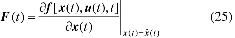
where ˆx denotes the estimate of state x, k represents the kth time step, superscripts − and + indicate the values before and after the update of measurement, respectively, P is covariance matrix, F is the Jacobians of function f with respect to the state vector x, which is given by

The update equations are responsible for computing a posteriori state estimate and for updating the covariance matrix, estimatebased on a priori which are as follows

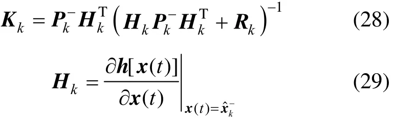
where K is Kalman gain matrix and H is the Jacobians of function h with respect to state vector x. Their equations are

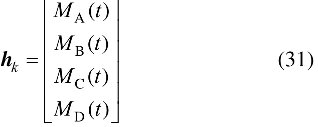
In the process model, one of the key kinetic parameters EKF. The system function fkfor estimatingand the heat released Qrare estimated by consists of Eqs. (2)-(5) and (30),

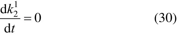
and the measurement function hkis given by

The system function fQfor estimating the heat released Qris a simplified reactor model given by Kittisupakorn [51] [see Eqs. (A1)-(A5) in Appendix] and the measurement function. The initial conditions and tuning parameters of the EKF for estimation ofand Qrare shown in Tables 3 and 4 [48].

3.3.3 Implementation of RTUMPC

The first step is to establish the criteria for model selection and model update. Since simplified model SM1 can deal with the largest set-point change in thethree simplified models, the value of SC1for SM1 is set to 1 °C, so that SM1 is selected to be used in the NMPC when the set-point change is larger than 1°C. SM2 is suitable to the set-point change smaller than SC1, and SM3 is suitable without set-point change. Furthermore, the maximum difference between the process output and the set point, limout, is set at 0.05 °C.

Table 3 Initial conditions and parameters for estimation of

Table 3 Initial conditions and parameters for estimation of

Initial values Parameters MA(0)=12 kmol P=diag[100, 10, 100, 100, 100] MB(0)=12 kmol MC(0)=0 kmol Q=diag[100, 1, 100, 1, 500] MD(0)=0 kmol k=38.9057 R=diag[10, 10, 10, 10] 12

Table 4 Initial conditions and parameters for estimation of Qr

A number of advanced process control algorithms have been introduced to improve the performance of batch reactor [47, 48, 52, 53]. To test the ability of the proposed algorithm to control batch processes, three popular control algorithms in literature are applied in this case study for comparison. They are LMPC algorithm, GMC algorithm and standard NMPC algorithm.

Figure 9 presents the control performance of four controllers for controlling the reactor temperature in a normal operation, with the start point set at 85 °C, since the four controllers behave almost the same in the time span from 0 to 17 min. The results show that the proposed RTUMPC and standard NMPC provide better performance than GMC and LMPC. Although LMPC provides a highest response speed, it also offers the largest overshoot, which may make the system unstable. It has been shown in literature that GMC presents good performance for tracking of one set point, but when applied to a system for tracking of a set-point profile, it may lead to relatively poor performance as illustrated in this case study. The main reason is that GMC needs a relatively long settling time. RTUMPC provides performance as good as the standard NMPC, largely due to its capability of model update according to the change of process condition. Fig. 10 shows that model update occurs when the set point has a large change in the RTUMPC, in which a more suitable model is selected as the prediction model to deal with the large set-point change. This is very important for the multiple model based predictive control algorithm to maintain the performance of controller. It should be noted that the standard NMPC controller designed in this study does not consider the computational cost for solution of control problem, which is an important issue that has to be considered in real industry. In these tests, the control problem for RTUMPC, NMPC and LMPC are formulated as Eqs. (1)-(4), and the prediction horizon P is set to 0.8 min, the control horizon M is set to 0.4 min, the weighting matrix Qwis 0.1, and Rwis 0.01.

Figure 9 Responses of controllers for normal operation

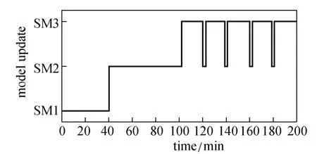
Figure 10 Time-varying model used in the RTUMPC for normal operation

The robustness aspects of the proposed RTUMPC are examined through simulation studies. In the three tests, the controller is used to control an operation where some of the conditions are changed from their nominal values in the operation. The first test is for model mismatch, with reaction constant k2decreasing 50%. The second test is for a reduction of 50% of heat-transfer coefficient from its nominal value, e.g., due to the fouling of heat-transfer surfaces. The third test is the combination of the two cases, with model mismatch and reduction of heat-transfer coefficient.

Figure 11 presents the control performance of the RTUMPC and the standard NMPC for the operation with model mismatch. The performance of the standard NMPC is a little worse than that of RTUMPC. With the model mismatch, the model built at the beginning of operation is inconsistent with the real process, so that the output of NMPC controller deviates from the real optimal value. As a result, the standard NMPC displays some offset from the set-point profile. The RTUMPC presents good performance, mainly due to the model update during the process operation, maintaining the accuracy of the modelalong the trajectory. As shown in Figs. 12 and 13, when the percentage variation of the estimated value of study, the simplified models are updated according tois larger than the tolerance εp, set at 12% in this current states and estimated value of update largely depends on the performance of state estimator for estimating the parameters of system. In addition, it presents one of the limitations for the application of RTUMPC algorithm: the state variables of the controlled system must be measurable or observable.

Figure 11 Responses of controllers for model mismatch

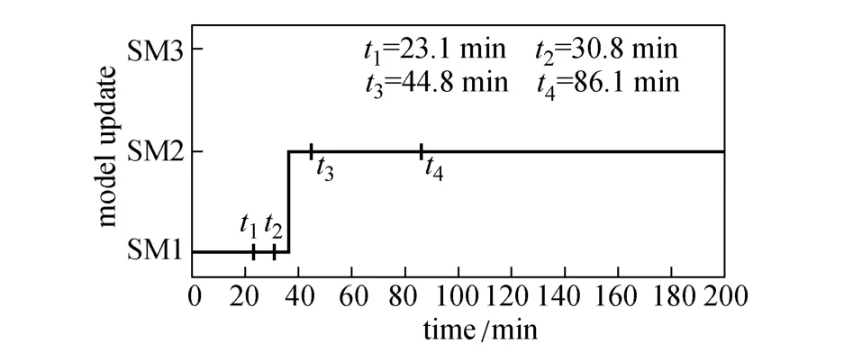
Figure 12 Time-vary model used in the RTUMPC for model mismatch

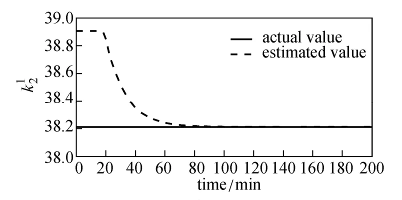
Figure 13 Estimate ofbased on EKF estimation

Figure 14 gives the responses of the controllers of standard NMPC and RTUMPC in response to a change in heat-transfer coefficient U, which reduces at the rate of 0.1 kW·m−2·°C−1per minute from the original value. The performance of the standard NMPC degrades much faster than that of RTUMPC. With the change of heat-transfer coefficient, the actual model of the system varies along the system trajectory, leading to worse performance of the standard NMPC. However, the performance of RTUMPC changes less, mainly because the RTUMPC keeps adjusting the model used as prediction model along the system trajectory to maintain perfect tracking of set-point profile.. The model

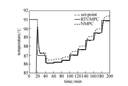
Figure 14 Responses of controllers for heat-transfer coefficient reduction [0.1 kW·m−2·°C−1per minute]

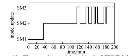
Figure 15 Time-varying model used in the RTUMPC for heat transfer coefficient change

Fig. 15 presents the process of model update in the control of the system. Although no model update occurs during the whole process operation, the RTUMPC still keeps good performance for tracking of set-point profile by selecting the most suitable model to be the prediction model. This further indicates that the simplified models used in RTUMPC have different performance in different operating regions and conditions.

Figure 16 presents the estimated value of heat released Qrbased on EKF. The difference between estimated value and actual value is getting larger with time, since the value of heat-transfer coefficient decreases. In addition, there are some transient squiggles for the estimated value of Qrat later stage, because the optimal trajectory of the system input, Tset, obtained by RTUMPC, presents some small and quick changes at later stage of the batch as shown in Fig. 17. However, this does not degrade the performance of RTUMPC, which further illustrates that the RTUMPC controller is much more robust with respect to the change in unmeasured parameters.

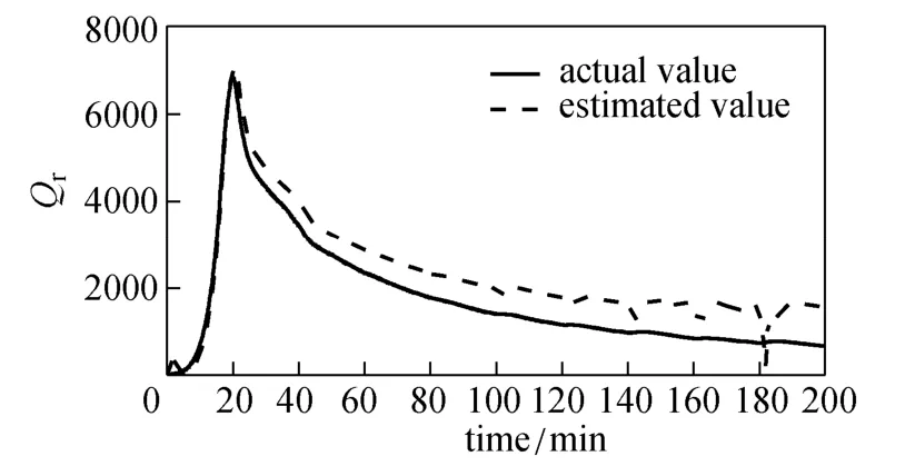
Figure 16 Estimated value of heat released Qrfor operation with heat-transfer coefficient change

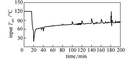
Figure 17 Optimal input of process for operation with heat-transfer coefficient change

Figure 18 gives the responses of the controller of RTUMPC for the third test in response to the perturbation of model mismatch and heat-transfer coefficient change. The performance of RTUMPC is good for the control. The process of model update and model selection is shown in Fig. 19, further illustrating the feasibility of the real-time model updated strategy.

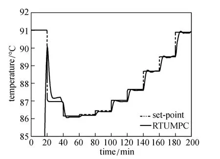
Figure 18 Responses of RTUMPC controller for model mismatch and heat-transfer coefficient change

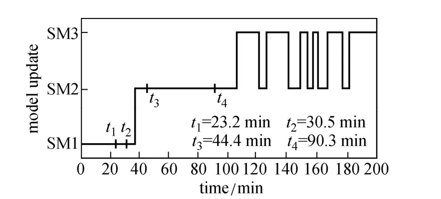
Figure 19 Time-varying model used in the RTUMPC for model mismatch and heat-transfer coefficient change

4 CONCLUSIONS

A real-time updated model predictive control strategy for batch processes is proposed, in which a batch process is reduced to a series of simplified models based on linearization method. Combined with a real-time model updated strategy, the models can automatically be selected and updated to be used in NMPC application. An exothermic batch reactor is used as a case study. Based on linearization technique, three simplified models are obtained to be used as the prediction model in NMPC. Based on these simplified models, the proposed real-time updated model predictive control algorithm is implemented in the process for performance evaluation. In the normal case test for realizing perfect tracking along the optimal trajectory, the RTUMPC provides similar performance to the standard NMPC, with better performance than LMPC and GMC. In addition, the RTUMPC is much more robust than the standard NMPC with respect to model mismatch and changes in unmeasured process parameters.

This strategy is generic and can be easily used in other batch processes for realizing perfect tracking of desired set-point trajectory in each cycle. It provides a reasonable compromise between the model prediction accuracy and the on-line computational time, which helps to facilitate the implementation of NMPC in industrial applications.

Future work can be addressed to find a more easy way to construct the selection and update criteria for real-time model updated strategy. A possible way for that is to find or design some key parameters, which can be easily measured, estimated or predicted, to drive the selection and update of the models. In addition, due to the similarity between the real-time updated model predictive control and real-time dynamic optimization (RTDO) from a mathematical point of view, an interesting way is to integrate the proposed strategy with RTDO to improve the performance of batch processes.

REFERENCES

1 Manenti, F., Rovaglio, M., “Integrated multilevel optimization in large-scale poly(ethylene terephthalate) plants”, Ind. Eng. Chem. Res., 47 (1), 92-104 (2007).

2 Zhang, R.D., Xue, A.K., Wang, S.Q., “Modeling and nonlinear predictive functional control of liquid level in a coke fractionation tower”, Chem. Eng. Sci., 66 (23), 6002-6013 (2011).

3 Zhou, M.F., Wang, S.Q., Jin, X.M., Zhang, Q.L., “Iterative learning model predictive control for a class of continuous/batch processes”, Chin. J. Chem. Eng., 17 (6), 976-982 (2009).

4 Lee, J.H., “Model predictive control: Review of the three decades of development”, Int. J. Control Autom., 9 (3), 415-424 (2011).

5 Özkan, L., Kothare, M.V., Georgakis, C., “Control of a solution copolymerization reactor using multi-model predictive control”, Chem. Eng. Sci., 58 (7), 1207-1221 (2003).

6 Huang, D.X., Wang, J.C., Jin, Y.H., “Stable MIMO constrained predictive control with steady state objective optimization”, Chin. J. Chem. Eng., 8 (4), 54-60 (2000).

7 Hermanto, M.W., Chiu, M.S., Braatz, R.D., “Nonlinear model predictive control for the polymorphic transformation of L-glutamic acid crystals”, AIChE J., 55 (10), 2631-2645 (2009).

8 Zhou, Z.Y., Yu, M., Wang, Z.Z., Liu, X.H., Guo, Y.Q., Zhang, F.B., Guo, Y., “Nonlinear model algorithmic control of a pH neutralization process”, Chin. J. Chem. Eng., 21 (4), 395-400 (2013).

9 Youqing, W., Donghua, Z., Furong, G., “Iterative learning model predictive control for multi-phase batch processes”, J. Process Control, 18 (6), 543-557 (2008).

10 Kansha, Y., Chiu, M.S., “Adaptive generalized predictive control based on JITL technique”, J. Process Control, 19 (7), 1067-1072 (2009).

11 Escano, J.M., Bordons, C., Vilas, C., Garcia, M.R., Alonso, A.A.,“Neurofuzzy model based predictive control for thermal batch processes”, J. Process Control, 19 (9), 1566-1575 (2009).

12 Henson, M.A., “Nonlinear model predictive control: Current status and future directions”, Comput. Chem. Eng., 23 (2), 187-202 (1998).

13 Biegler, L.T., “Efficient solution of dynamic optimization and NMPC problems”, In: Nonlinear Model Predictive Control, Allgower, F., Zheng, A., eds., Birkhauser, Basel, 219-243 (2000).

14 Schäfer, A., Kühl, P., Diehl, M., Schlöder, J., Bock, H.G., “Fast reduced multiple shooting methods for nonlinear model predictive control”, Chemical Engineering and Processing: Process Intensification, 46 (11), 1200-1214 (2007).

15 Sun, F., Zhong, W.M., Cheng, H., Qian, F., “Novel control vector parameterization method with differential evolution algorithm and its application in dynamic optimization of chemical processes”, Chin. J. Chem. Eng., 21 (1), 64-71 (2013).

16 Liu, X.G., Chen, L., Hu, Y.Q., “Solution of chemical dynamic optimization using the simultaneous strategies”, Chin. J. Chem. Eng., 21 (1), 55-63 (2013).

17 Zavala, V.M., Laird, C.D., Biegler, L.T., “Fast implementations and rigorous models: Can both be accommodated in NMPC?”, International Journal of Robust and Nonlinear Control, 18 (8), 800-815 (2008).

18 Zavala, V.M., Biegler, L.T., “Optimization-based strategies for the operation of low-density polyethylene tubular reactors: Nonlinear model predictive control”, Comput. Chem. Eng., 33 (10), 1735-1746 (2009).

19 Cannon, M., Ng, D., Kouvaritakis, B., “Successive linearization NMPC for a class of stochastic nonlinear systems”, In: Nonlinear Model Predictive Control, Magni, L., Raimondo, D.M., Allgower, F., Zheng, A., eds., Springer, Berlin Heidelberg, 249-262 (2009).

20 Nagy, Z.K., “Model based control of a yeast fermentation bioreactor using optimally designed artificial neural networks”, Chem. Eng. J., 127 (1-3), 95-109 (2007).

21 Bao, Z., Pi, D., Sun, Y., “Nonlinear model predictive control based on support vector machine with multi-kernel”, Chin. J. Chem. Eng., 15 (5), 691-697 (2007).

22 Lu, M., Jin, C.B., Shao, H.H., “An improved fuzzy predictive control algorithm and its application to an industrial CSTR process”, Chin. J. Chem. Eng., 17 (1), 100-107 (2009).

23 Kuure-Kinsey, M., Bequette, B.W., “Multiple model predictive control of nonlinear systems”, In: Nonlinear Model Predictive Control, Magni, L., Raimondo, D.M., Allgower, F., Zheng, A., eds., Springer, Berlin Heidelberg, 153-165 (2009).

24 Kuure-Kinsey, M., Bequette, B.W., “Multiple model predictive control strategy for disturbance rejection”, Ind. Eng. Chem. Res., 49 (17), 7983-7989 (2010).

25 Peterson, T., Hernández, E., Arkun, Y., Schork, F.J., “A nonlinear DMC algorithm and its application to a semibatch polymerization reactor”, Chem. Eng. Sci., 47 (4), 737-753 (1992).

26 Dougherty, D., Cooper, D., “A practical multiple model adaptive strategy for multivariable model predictive control”, Control Eng. Prac., 11 (6), 649-664 (2003).

27 Wang, F.Y., Bahri, P., Lee, P.L., Cameron, I.T., “A multiple model, state feedback strategy for robust control of non-linear processes”, Comput. Chem. Eng., 31 (5-6), 410-418 (2007).

28 Bonis, I., Xie, W., Theodoropoulos, C., “A linear model predictive control algorithm for nonlinear large-scale distributed parameter systems”, AIChE J., 58 (3), 801-811 (2012).

29 Dones, I., Manenti, F., Preisig, H.A., Buzzi-Ferraris, G., “Nonlinear model predictive control: A self-adaptive approach”, Ind. Eng. Chem. Res., 49 (10), 4782-4791 (2010).

30 Su, Q.L., Braatz, R.D., Chiu, M.S., “Concentration control for semi-batch Ph-shift reactive crystallization of L-glutamic acid”, In: Proceedings of the 8th IFAC Symposium on Advanced Control of Chemical Processes, Kariwala, V., Samavedham, L., Braatz, R.D., eds., Elsevier, Singapore, 228-233 (2012).

31 Bonvin, D., “Control and optimization of batch processes”, Control Systems, IEEE, 26 (6), 34-45 (2006).

32 Terwiesch, P., Agarwal, M., “A discretized nonlinear state estimator for batch processes”, Comput. Chem. Eng., 19 (2), 155-169 (1995).

33 Tatiraju, S., Soroush, M., Ogunnaike, B.A., “Multirate nonlinear state estimation with application to a polymerization reactor”, AIChE J., 45 (4), 769-780 (1999).

34 Rui, H., Patwardhan, S.C., Biegler, L.T., “Stability of a class of discrete-time nonlinear recursive observers”, J. Process Control, 20 (10), 1150-1160 (2010).

35 Peters, N., Guay, M., DeHaan, D., “Real-time dynamic optimization of batch systems”, J. Process Control, 17 (3), 261-271 (2007).

36 Bequette, B.W., “Nonlinear control of chemical processes: A review”, Ind. Eng. Chem. Res., 30 (7), 1391-1413 (1991).

37 Liu, T., Gao, F.R., Industrial Process Identification and Control Design, Springer, London, 433-452 (2012).

38 Luyben, M.L., Tyreus, B.D., Luyben, W.L., “Plantwide control design procedure”, AIChE J., 43 (12), 3161-3174 (1997).

39 Skogestad, S., “Control structure design for complete chemical plants”, Comput. Chem. Eng., 28 (1-2), 219-234 (2004).

40 Xiao, J., Huang, Y.L., Liu, Z., “Proactive product quality control: An integrated product and process control approach to MIMO systems”, Chem. Eng. J., 149 (1-3), 435-446 (2009).

41 Yuan, Z.H., Chen, B.Z., Zhao, J.S., “Effect of manipulated variables selection on the controllability of chemical processes”, Ind. Eng. Chem. Res., 50 (12), 7403-7413 (2011).

42 McGahey, S.L., Cameron, I.T., “A multi-model repository with manipulation and analysis tools”, Comput. Chem. Eng., 31 (8), 919-930 (2007).

43 Gattu, G., Zafiriou, E., “Nonlinear quadratic dynamic matrix control with state estimation”, Ind. Eng. Chem. Res., 31 (4), 1096-1104 (1992).

44 Sistu, P.B., Bequette, B.W., “Nonlinear model-predictive control: Closed-loop stability analysis”, AIChE J., 42 (12), 3388-3402 (1996).

45 Meadows, E.S., Rawlings, J.B., Nonlinear Process Control, Prentice Hall, PTR, London, 233-310 (1997).

46 Mayne, D.Q., Rawlings, J.B., Rao, C.V., Scokaert, P.O.M., “Constrained model predictive control: Stability and optimality”, Automatica, 36 (6), 789-814 (2000).

47 Cott, B.J., Macchietto, S., “Temperature control of exothermic batch reactors using generic model control”, Ind. Eng. Chem. Res., 28 (8), 1177-1184 (1989).

48 Arpornwichanop, A., Kittisupakorn, A., Mujtaba, I.M., “On-line dynamic optimization and control strategy for improving the performance of batch reactors”, Chem. Eng. Process., 44 (1), 101-114 (2005). 49 Yildiz, U., Gurkan, U.A., Ozgen, C., Leblebicioglu, K., “State estimator design for multicomponent batch distillation columns”, Chem. Eng. Res. Des., 83 (A5), 433-444 (2005).

50 Sirohi, A., Choi, K.Y., “On-line parameter estimation in a continuous polymerization process”, Ind. Eng. Chem. Res., 35 (4), 1332-1343 (1996).

51 Kittisupakorn, P., “The use of nonlinear model predictive control techniques for the control of a reactor with exothermic reactions”, Ph.D. Thesis, University of London, UK (1995).

52 Arpornwichanop, A., Kittisupakorn, P., Hussain, M.A., “Model-based control strategies for a chemical batch reactor with exothermic reactions”, Korean J. Chem. Eng., 19 (2), 221-226 (2002).

53 Mujtaba, I.M., Aziz, N., Hussain, M.A., “Neural network based modelling and control in batch reactor”, Chem. Eng. Res. Des., 84 (8), 635-644 (2006).

APPENDIX

Simplified model equations for Qrestimation

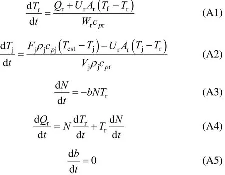
where Wr=1560 kg, cpr=1.8828 kJ·kmol−1·°C−1, Ur=40.842 kW·m−2·°C−1, and Ar=6.24 m2.

PROCESS SYSTEMS ENGINEERING AND PROCESS SAFETY

Chinese Journal of Chemical Engineering, 22(3) 318—329 (2014)

10.1016/S1004-9541(14)60057-4

2013-03-23, accepted 2013-05-23.

*Supported by the National Natural Science Foundation of China (21136003，21176089), the National Science &Technology Support Plan (2012BAK13B02), the National Major Basic Research Program (2014CB744306), the Natural Science Foundation Team Project of Guangdong Province (S2011030001366), and the Fundamental Research Funds for Central Universities (2013ZP0010).

**To whom correspondence should be addressed. E-mail: ceyuqian@scut.edu.cn