Influence of artificial ecological floating beds on river hydraulic characteristics*

RAO Lei (饶磊)

College of Mechanical and Electronic Engineering, Hohai University, Changzhou 213022, China,

E-mail: rao_lei@163.com

QIAN Jin (钱进), AO Yan-hui (敖燕辉)

Key Laboratory of Integrated Regulation and Resource Development on Shallow Lakes, Ministry of Education, College of Environment, Hohai University, Nanjing 210098, China

Influence of artificial ecological floating beds on river hydraulic characteristics*

RAO Lei (饶磊)

College of Mechanical and Electronic Engineering, Hohai University, Changzhou 213022, China,

E-mail: rao_lei@163.com

QIAN Jin (钱进), AO Yan-hui (敖燕辉)

Key Laboratory of Integrated Regulation and Resource Development on Shallow Lakes, Ministry of Education, College of Environment, Hohai University, Nanjing 210098, China

(Received March 21, 2014, Revised April 28, 2014)

The artificial ecological floating bed is widely used in rivers and lakes to repair and purify polluted water. However, the water flow pattern and the water level distribution are significantly changed by the floating beds, and the influence on the water flow is different from that of aquatic plants. In this paper, based on the continuous porous media model, a moveable two-layer combination model is built to describe the floating bed. The influences of the floating beds on the water flow characteristics are studied by numerical simulations and experiments using an experimental water channel. The variations of the water level distribution are discussed under conditions of different flow velocities (v=0.1 m/s, 0.2 m/s, 0.30 m/s, 0.4 m/s), floating bed coverage rates (20%, 40%, 60%) and arrangement positions away from the channel wall (D=0 m, 0.1 m, 0.2 m). The results indicate that the flow velocity increases under the floating beds, and the water level rises significantly under high flow velocity conditions in the upstream region and the floating bed region. In addition, the average rising water level value (ARWLV) increases significantly with the increase of the floating bed coverage rate, and the arrangement position of floating beds in the river can also greatly influence the water level distribution under a high-flow velocity condition (v≥0.2 m/s).

ecological floating bed, flow pattern, rising water level, numerical simulation

Introduction

The artificial ecological floating bed is a commonin situtreatment technique for repairing and purifying polluted surface water. The implementation practice indicates that ecological floating beds can effectively purify water and significantly enhance the self-repair ability of rivers and lakes[1-3]. With the biological purification method, the pollutants in the water can be absorbed by the plants of the floating bed through their root system, and also be degraded by themicroorganisms that have parasitized the root systems[4]. In general, the purifying efficiency of the ecological floating bed generally increases with the plant density and the total area of the floating beds[5,6]. However, the blocking of the water flow limits the application range of the technique, especially in some flood discharge river channels.

In recent years, the hydrodynamic influence of aquatic plants on rivers was amply studied. Based on interior or outdoor experiments and hydromechanic studies, the drag coefficient of the submerged plants of emergent plants and floating plants in the water flow was determined[7-10], and the influence of the aquatic plant density on the water level distribution was analyzed[11-14]. However, the impacts of the floating beds on the water flow characteristics were not well covered.

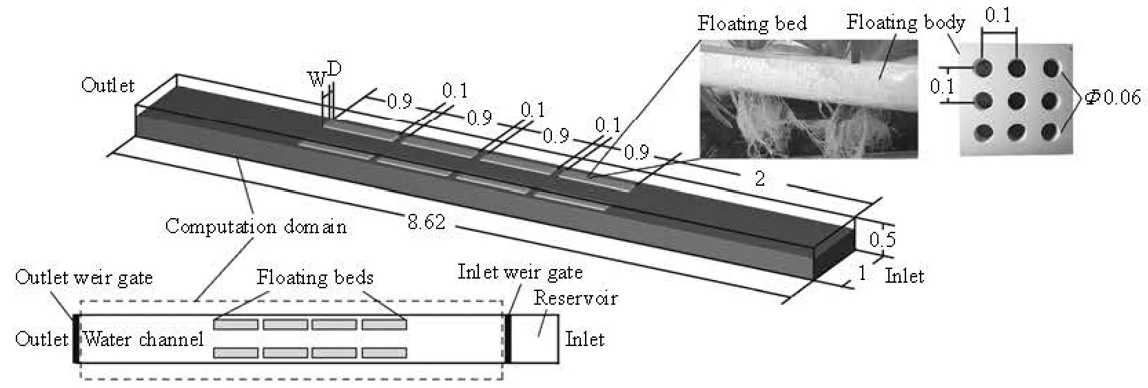
Fig.1 Sketch of the experimental channel and the computational domain (m)

A floating bed usually includes three layers, the upper leaf and the stem of plants, the middle floating body and the bottom root system. Thus, the influence of the floating bed on the water flow is different from that of aquatic plants and has some special characteristics. First, the floating bed can move freely with the water surface fluctuation with a fixed position related to the river bank. Secondly, the floating body is made of a light waterproof material, but the root system is of a porous structure. The water can flow into the root system region but be completely blocked by the floating body. Thus, their motion with the water flow should also be taken into account in the simulation modeling.

In this work, based on the continuous porous media model, a two-layer combination model is built to describe the floating bed, and the influences of the floating beds on the water flow characteristics are studied by numerical simulations and experiments in an experimental water channel. In addition, the variations of the water level distribution are discussed under conditions of different flow velocities (v=0.1 m/s, 0.2 m/s, 0.3 m/s, 0.4 m/s), floating bed coverage rates (20%, 40%, 60%) and arrangement positions (D= 0 m, 0.1 m, 0.2 m).

1. Physical models

1.1Experimental equipment and computational do

main

In this work, a water channel of rectangular section is used to simulate a natural river, and eight floating beds are arranged in the middle region of the channel. The sketch of the experimental channel and the dimension of the computational domain are shown in Fig.1. The water channel is fixed on a cement base with a 0.1odip angle along the length direction. The water flow in the channel is driven by a circulating water pump, and the flow velocity in the channel can be controlled by the pump and the accessory valve system. To eliminate the inlet velocity fluctuation, the water is pumped into the reservoir first and then flows into the water channel through an inlet weir gate between the reservoir and the channel. At the outlet side of the channel, a moveable outlet weir gate is used to control the water level of the channel. The floating beds in this work are made of polystyrene foamed plastic slabs withIris tectorum.The polystyrene foamed plastic slabs are used as the floating body, and there are several holes ofφ0.06 m spaced 0.1 m apart on the slabs. TheIris tectorumis planted in the holes and grow in the water until the root system is developed. Each floating bed is fixed on the side wall of the channel with a thin rope and can move up and down with the water level fluctuation at the same position.

Fig.2 The physical model of the floating bed (m)

1.2The floating bed model

In the three-layer structure of the floating bed, the leaves and the stem of the plants are neglected in the physical model as they are always above the water surface. Because of the different physical properties of the floating body and the root system, the floating bed is described as a combination body including two layers. The sketch of the combination model is shown in Fig.2. The floating body is treated as a solid model with waterproof boundaries in the calculation. The root system is assumed to be a continuous porous medium, with possible flow in this region. The additional drag resistance of the root system is taken into account by the permeability of the root system region[15]. To simplify the calculation, the following assumptions are made:

(1) The drag coefficient of the root system to the water flow is isotropic.

(2) The dimension of the root system region is unchanged in the calculation, and the root swing phenomenon in the water flow is neglected.

2. Numerical models

2.1Governing equations

In this study, the water density is assumed to be a constant. Then, the continuity equation can be written as follows

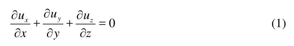
whereux,uyanduzrepresent the velocity components inx,yandzdirections.

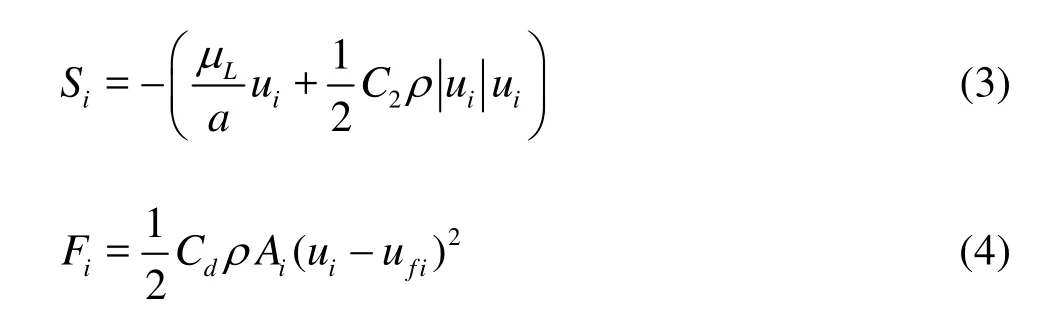
For describing the water flow in the root system region, an additional source item is added in the Navier-Stokes equations to describe the drag resistance of the root system to the water flow. The momentum equations are as follows[15,16]

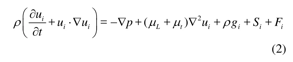
whereρis the density of the water,uiis the velocity,tis the time,pis the time-averaged pressure,giis the acceleration of gravity,μLis the molecular viscosity coefficient,tμis the turbulence eddy viscous coefficient of the water.Siis the additional source item of the drag resistance of the root system, which is described by the momentum variation due to the viscosity and the inertia of the fluid in the continuous porous media.iFis the coupling source item which describes the momentum exchange between the floating bed and the flow[17]. whereI/ais the viscosity drag coefficient,C2is the inertia drag coefficient. Based on the Darcy’s law, these two parameters can be obtained from experiments,Cdis the comprehensive resistance coefficient of the floating bed,iAis the projected area on each coordinate plane,ufiis the velocity of the floating bed.

The floating beds can produce a turbulent flow in the channel. Here, thek-εequations are used:

wherekis the turbulence kinetic energy,εis the dissipation rate of the turbulence kinetic energy.kσandεσare the Prandtl numbers corresponding tokandε, respectively.σ1εandσ2εare empirical constants. In this work,σk=1.0,σε=1.3,σ1ε=1.44 andσ2ε=1.92.Gkis the turbulent kinetic energy produced by the gradient of the average velocity, which can be described as follows

Fromkandε, the turbulence eddy viscous coefficient of the watertμcan be expressed as follows

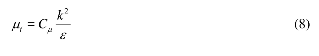
whereCμis an empirical constant. Here,Cμ=0.09.

2.2VOF model

To study the water level distribution in the channel, the volume of fluid (VOF) model is used to simulate the motion interface between air and water. The continuous equation of the volume fraction of the water phase or the air phase can be written as follows

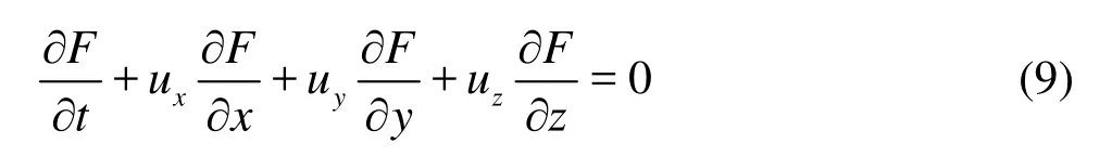
whereFis the volume function for the water phase and the air phase. In each element mesh, the sum ofthe water and air fractions is 1. Based on theFfunction, the free surface of the water flow can be constructed and traced.

2.3The motion control equation of floating bed

The floating beds only have one degree of freedom (DOF) inzdirection, without DOFs inx,ydirections and all rotational DOFs. Thus, the motion control equation of the floating bed inzdirection can be written as follows

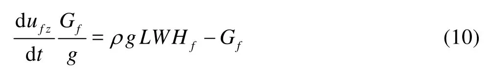
whereuf zis the velocity component of the floating bed inzdirection,Gfis the weight of a piece of the floating bed,LandWare the length and the width of the floating bed, respectively.Hfis the immersion depth of the floating bed.

2.4Boundary conditions

The inlet flow velocity is taken as the inlet boundary condition, and the value is the average velocity at the inlet side of the channel, which is measured with an acoustic Doppler velocimeter (ADV). In addition, the values ofkandεof the inlet flow can be calculated using the following empirical equations[17]

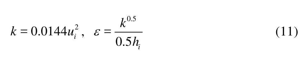
whereuiandhiare the inlet average velocity and the hydraulic head of the inlet side, respectively. In addition, the outlet of the water channel is taken as the outflow boundary, and an atmosphere pressure is assumed on the interface between water and air. Furthermore, the two side walls and the bottom of the water channel are taken as the no-slip wall boundary in the calculation. About 720 000 hexahedral grids are used for the model, and the time step is 0.002 s.

3. Simulation and experiment results and analyses

3.1Physical experiments

To study the flow velocity and the water level distribution under the influence of the floating beds, a series of experiments were performed under conditions of different inlet velocities (v=0.1 m/s, 0.2 m/s, 0.3 m/s, 0.4 m/s), floating bed coverage rates (20%, 40%, 60%) and arrangement position conditions (D= 0 m, 0.1 m, 0.2 m). From 1 m to 7.5 m in the length direction of the channel, 14 sampling cross sections of 0.5 m apart between each other are selected. The water depth and the flow velocity are measured on these sampling cross sections (Fig.3 shows the position of the sampling points on a section). In addition, to avoid uncertainty during the water depth and flow velocity measurements, a statistical average method is used.

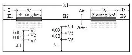
Fig.3 The position of sampling points on the cross section (m)

In Fig.3,Wis the width of the floating bed,Dis the distance between the floating bed and the channel wall. When the water flow is in a stable state, the water depths at points “H1”, “H2” and “H3” are measured by a ruler, and the recorded average fluid depth in this section is the average value for these three points. In addition, the flow velocities at points “V1” to “V6” are measured using an ADV. The depth average velocity under the floating bed and at the middle of the channel in this section is represented by the average velocity value of points “V1” to “V3” and “V4”to “V6”, respectively. In addition, the height of the outlet weir gate is 0.306 m in the experiment.

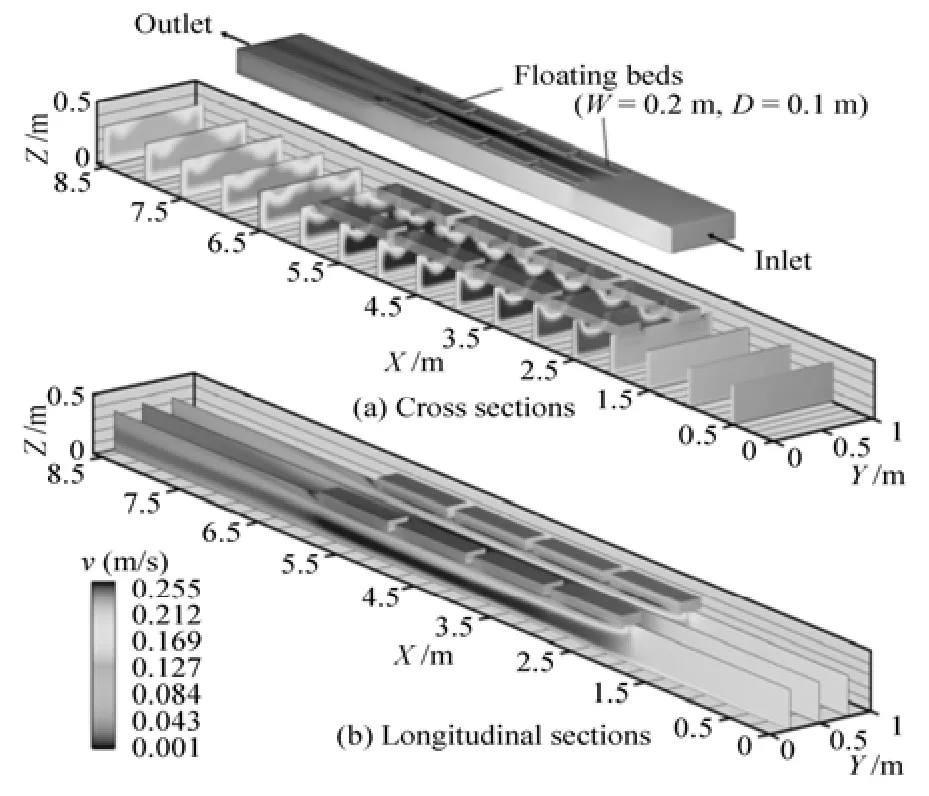
Fig.4 The velocity distribution in the channel

3.2The flow velocity distribution

Under the influence of the floating beds, the flow pattern in the channel is more complex than the common water flow. The flow velocity distribution in the channel under the 0.2 m/s inlet velocity condition isshown in Fig.4.

Figure 4 shows that the flow velocity distribution in the channel is non-uniform, especially, in the floating bed region. Because the floating beds impede the flow through the area in the floating bed region, the flow velocity increases sharply when the water flows into this region. In the cross-section of the channel, the flow velocity at the middle of the channel is higher than at the two sides. Under the influence of the drag resistance of the root system, the flow velocity in the root system is very small, and the water flow under the floating beds is greatly influenced by the root system. The flow velocity vector map and the depth average velocity() distribution along the flow direction for describing the characteristics of the flow pattern under the floating beds are shown in Fig.5.

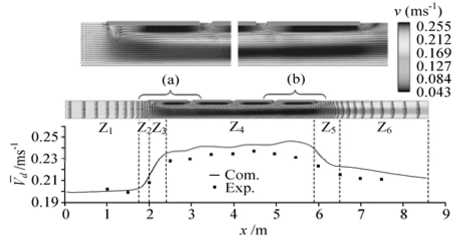
Fig.5 The velocity distribution under floating beds (m)

In Fig.5, there are six regions marked with “Z1”to “Z6” from the inlet to the outlet of the channel. The “Z1” region is the starting section of the water flow. The flow velocity in this section is almost invariant and uniform, and the average velocity is approximately equal to the inlet velocity. In the “Z2” region, the water flow begins to be blocked by the floating beds. The upper layer of the water flow tends to mix into the bottom layer, and the depth average velocity begins to increase in this region. The “Z3” region is the front section of the first piece of the floating beds, and the flow pattern changes greatly in this region. The main stream of the water flow passes through the bottom of the root system region, and the flow velocity increases quickly in this bottom region. Moreover, a small part of the water flows into the root system region (Fig.5(a)). Because of the drag effect of the root system on the flow, the flow velocity decreases quickly in the root system region within a short distance. In the “Z4” region, the main stream of the water flow is narrowly compressed by the floating beds, and the flow velocity increases significantly. In addition, an eddy is generated at the gaps of the floating beds, and these gaps can enhance the convection between the upper and bottom layers of the water flow, and it is helpful to improve the pollutant absorbing efficiency of the root system. The “Z5” is the wake flow influence region of the floating beds. Under the pressure difference between the upper and bottom layers in this region, a small part of the bottom water flow begins to flow into the upper layer, and it makes the depth average velocity decrease quickly (Fig.5(b)). The “Z6” region is the flow structure recovering region. The flow velocity distribution tends to be uniform, and the depth average velocity decreases slightly with the increase of the distance to the floating beds region.

3.3Water level distribution

The water level is a very important indicator of a river to describe its flow state. The water level distribution and the average fluid depth (Hf) along the flow direction in the channel are shown in Fig.6.

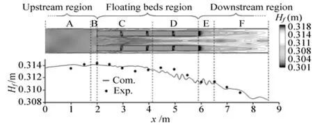
Fig.6 The water level distribution and the average fluid depth

In Fig.6, based on the water level variations along the flow direction, the water channel is separated into six regions marked by “A” to “F”, respectively. The regions “A” and “B” belong to the upstream region of the channel. Under the influence of the floating beds, the water level in this region is obviously higher than that of the downstream region, and the average fluid depth takes the maximum value in the “B” region. The “C” and “D” regions are in the floating bed region. The average fluid depth slightly drops in this region. In the “C” region, the water flow is suddenly limited within the narrow way between two rows of the floating beds. This results in a quick increase of the turbulence intensity and the flow resistance in this region. Thus, the water level in this region remains at a high level. However, in the “D” region, with the flow velocity under the floating beds increasing, the average fluid depth decreases slowly. In the “E” region because of the influence of the wake flow of the floating beds, the water level behind the floating beds is very low, but it is high in the middle of the channel. Because of the influence of the turbulent flow in this region, the average fluid depth fluctuates greatly. The “F” region sees the flow pattern recovering, where the water level is gradually recovered to the initial state.

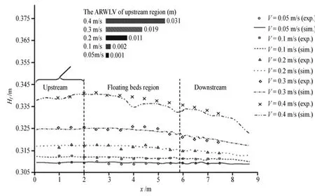
Fig.7 The average fluid depth distribution and the ARWLV in upstream region at different flow velocities

4. Discussions

In natural rivers, the influence of the floating beds on the river flow pattern is complicated under various conditions. In this study, under conditions of different flow velocities, coverage rates and arrangement position conditions, the water level distribution varies in the following manner.

4.1Water level variation under different flow velocities

In the flood period, the flood carrying capacity of a river influences the safety of cities. The influence of the floating beds on the flood carrying capacity of a river is a particular concern in recent years. In this work, based on the same floating bed model (W= 0.2 m,D=0.1 m), the water level distributions are studied in the experimental channel at different flow velocities. The average rising water level value (ARWLV) is introduced to indicate the influence extent of the floating bed on the water level, and it can be calculated as follows

whereHnoris the average fluid depth without the floating beds. Figure 7 shows the average fluid depth variation curve along the flow direction, and the ARWLV of the upstream region at different flow velocities are also shown.

When the inlet flow velocity is below 0.1 m/s, the distribution of the average fluid depth along the flow direction is uniform, and the ARWLV of the upstream region is below 0.0023 m. In this low-flow velocity situation, the influence of the floating beds can be neglected. When the inlet flow velocity increases to 0.3 m/s, the water levels of the upstream region and the floating beds region obviously increase, and the ARWLV of the upstream region can reach 0.0188 m in this situation. When the inlet velocity increases to 40 cm/s, the ARWLV of the upstream region increases sharply and the value reaches 0.0314 m. The results indicate that the floating beds can increase the water level significantly, and the ARWLV of the upstream region increases quickly with the increase of the flow velocity.

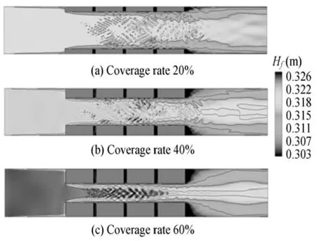
Fig.8 Water level distribution at different coverage rates of floating beds (inlet flow velocity is 0.2 m/s)

4.2Water level distribution at different coverage rates

The high coverage rate of the floating beds is beneficial in terms of facilitating its root system to absorb more pollutants from water, but it increases the resistance to the water flow. In this study, three coverage rates of the floating beds are considered in the experiments. The coverage rate is calculated by the rate of the total area of the floating beds and the water area in the floating bed region. Figure 8 shows the water level distribution at different coverage rates, andthe relations between the ARWLV of the upstream region and the flow velocity at different coverage rates are shown in Fig.9.

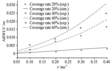
Fig.9 Relation between the ARWLV of the upstream region and the flow velocity at different coverage rates

When the coverage rate is below 20%, the gap between the two rows of the floating beds is wide enough. Thus, the water flow can pass through the floating bed region with little resistance, and the water level difference in the channel is small (Fig.8(a)). In this situation, the ARWLV of the upstream region increases slightly with the increase of the flow velocity. Even at a flow velocity of 0.4 m/s , the ARWLV of the upstream region is only approximately 0.003 m (Fig.9). When the coverage rate is above 40%, the flow capacity in the floating bed region is far below that in the 20% situation, it makes the water level in the upstream and floating bed regions increase significantly (Figs.8(b), 8(c)). Figure 9 shows that the ARWLV of the upstream region increases quickly with the flow velocity when the coverage rate is above 40%. The results indicate that the blocking effect of the floating bed to the water flow is influenced by the coverage rate greatly. Especially under high-flow velocity conditions, the ARWLV of the upstream region increases sharply with the coverage rate.

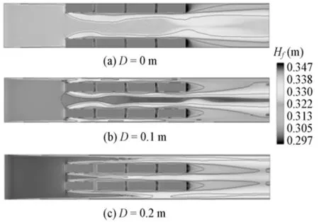
Fig.10 Water level distribution for different arrangement positions (inlet flow velocity is 0.4 m/s)

4.3Water level distribution for different arrangement positions

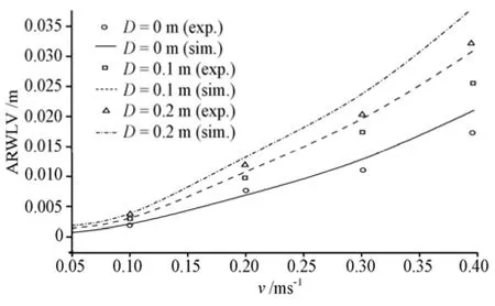
Fig.11 The relation between the ARWLV of the upstream region and the flow velocity for different arrangement positions

In practice, the arrangement position of the floating beds is always considered from the view of scenery. For studying the influence of the arrangement of the floating beds on the water level distribution, different distances between the floating beds and the channel wall are considered. Figure 10 shows the water level distributions for different arrangement positions, and the relations between the ARWLV of the upstream region and the velocity for different arrangement positions are shown in Fig.11. channel wall (D=0 m), the water flow can pass through the gap between two rows of the floating beds with little resistance (Fig.10(a)). However, if the floating beds are arranged apart from the channel wall with a distance, and the upper layer water flow is separated to three streams by the floating beds (Figs.10(b), 10(c)). The resistance to the water flow generally increases with the decrease of the maximum gap width between the floating beds and the channel walls. Thus, the water level distribution in theD= 0.2 m situation is more non-uniform than in the other situation. In addition, Fig.11 shows that the influence extent of the arrangement position on the ARWLV of the upstream region increases with the increase of the flow velocity. Under the same 0.4 m/s flow velocity condition, the ARWLV of the upstream region can increase from 0.0168 m to 0.0325 m when the arrangement position changes fromD=0 m mode toD= 0.2 m mode.

Figure 10 shows that the water level distribution is different among three types of arrangement positions. When the floating beds are arranged against the

5. Conclusions

This paper discusses the influence of ecological floating beds on the water flow pattern under variousconditions in the experimental channel, and the results are summarized as follows:

(1) The two-layer combination model can descrybe well the structural characteristics of the floating bed, and the simulation results are in agreement with the experimental results.

(2) The influence of the floating bed on the water level is weak under low-flow velocity conditions with the flow velocity lower than 0.1 m/s, but the ARWLV of the upstream region increases quickly with the flow velocity.

(3) A high coverage rate can obviously increase the ARWLV of the upstream region and then decrease the flow capacity of the river significantly when the flow velocity is higher than 0.2 m/s. And the extent of this influence increases as the flow velocity increases.

(4) The arrangement position is an important factor influencing the flow capacity of the river. The ARWLV of the upstream region increases with the decrease of the maximum gap width between the floating beds and the channel walls, and the influence extent of the arrangement is more significant under a high-flow velocity condition (v≥0.2 m/s).

These results show that the floating bed can change the flow pattern, decrease the river flow capacity and raise the water level. To decrease the negative effects on the flow capacity of a river, the coverage rate should be controlled within a reasonable range, and the floating beds should be arranged against the river bank as far as possible.

[1] ZHOU Xiao-hong, WANG Guo-xiang. Nutrient concentration variations during oenanthe javanica growth and decay in the ecological floating bed system[J].Journal of Environmental Sciences,2010, 22(11): 1710-1717.

[2] XIAN Q., HU L. and CHEN H. et al. Removal of nutrients and veterinary antibiotics from swine wastewater by a constructed macrophyte floating bed system[J].Journal of Environmental Management,2010, 91(12): 2657-2661.

[3] LI X.-N., SONG H.-L. and LI W. et al. An integrated ecological floating-bed employing plant, freshwater clam and biofilm carrier for purification of eutrophic water[J].Ecological Engineering,2010, 36(4): 382-390.

[4] SUN L., LIU Y. and JIN H. Nitrogen removal from polluted river by enhanced floating bed grown canna[J].Ecological Engineering,2009, 35(1): 135-140.

[5] CAO Wen-ping, WANG Bing-bing. Application status quo and development direction of ecological floating bed[J].Industrial Water Treatment,2013, 33(2): 5-9(in Chinese).

[6] HUANG L., ZHUO J. and GUO W. et al. Tracing organic matter removal in polluted coastal wasters via floating bed phytoremediation[J].Marine pollution Bulletin,2013, 71(1-2): 74-82.

[7] HUAI Wen-xin, ZHAO Lei and LI Dan et al. Experimental analysis of vertical profiles of stream-wise velocities in flows through vegetation with PIV[J].Journal of Experiments in Fluid Mechanics,2009, 23(1): 26-30(in Chinese).

[8] STOESSER T., SALVADOR G. and RODI W. et al. Large eddy simulation of turbulent flow through submerged vegetation[J].Transport in Porous Media,2009, 78(3): 347-365.

[9] HUAI Wen-xin, WU Zhen-lei and QIAN Zhong-dong et al. Large eddy simulation of open channel flows with non-submerged vegetation[J].Journal of Hydrodynamics,2011, 23(2): 258-264.

[10] KOTHYARI U. C., HAYASHI K. and HASHIMOTO H. Drag coefficient of unsubmerged rigid vegetation stems in open channel flows[J].Journal of Hydraulic Research,2009, 47(6): 691-699.

[11] WANG C., WANG P. Hydraulic resistance characteristics of riparian reed zone in river[J].Journal of Hydrologic Engineering,2007, 12(3): 267-272.

[12] SANJOU M., NEZU I. Turbulence structure and coherent motion in meandering compound open-channel flows[J].Journal of Hydraulic Research,2009, 47(5): 598-610.

[13] ZHU Hong-jun, ZHAO Zhen-xing. Influences of cropping loops in ecological river on hydraulic behavior of flow[J].Hydro-Science and Engineering,2007, (1): 31-35(in Chinese).

[14] WANG Pei-fang, WANG Chao and ZHU David Z. et al. Hydraulic resistance of submerged vegetation related to effective height[J].Journal of Hydrodynamics, 2010, 22(2): 265-273.

[15] XU Z. H., MA G. W. and LI S. C. A graph theoretic pipe network method for water flow simulation in a porous medium: GPNM[J].International Journal of Heat and Fluid Flow, 2014, 45(2): 81-97.

[16] ALVES B., BARLETTA A. and HIRATA S. et al. Effects of viscous dissipation on the convective instability of viscoelastic mixed convection flows in porous media[J].International Journal of Heat and Mass Transfer,2014, 70(3): 586-598.

[17] WU Shi-qiang, TONG Zhong-shan and ZHOU Hui et al. Simulation methods for accumulation patterns floating debris in hydropower stations[J].Advance in Science and Technology of Water Resources,2010, 30(2): 24-28.

10.1016/S1001-6058(14)60054-8

* Project supported by the Major Science and Technology Program for Water Pollution Control and Treatment (Grant No. 2012ZX07101-008), the National Science Fund for Distinguished Young Scholars (Grant No. 51225901), the Research Fund for Innovation Team of Ministry of Education (Grant No. IRT13061) and the Jiangsu Province QingLan Project.

Biography: RAO Lei (1975-), Male, Ph. D.,

Associate Professor