Effect of Spatial and Temporal Scales on Habitat Suitability Modeling: A Case Study of Ommastrephes bartramii in the Northwest Pacific Ocean

GONG Caixia, CHEN Xinjun,, GAO Feng, and TIAN Siquan

1) College of Marine Sciences, Shanghai Ocean University, Shanghai 201306, P. R. China

2) The Key Laboratory of Sustainable Exploitation of Oceanic Fisheries Resources, Ministry of Education, Shanghai 201306, P. R. China

3) International Center for Marine Sciences, Shanghai Ocean University, Shanghai 201306, P. R. China

Effect of Spatial and Temporal Scales on Habitat Suitability Modeling: A Case Study of Ommastrephes bartramii in the Northwest Pacific Ocean

GONG Caixia1),2),3), CHEN Xinjun1),2),3),*, GAO Feng1),2),3), and TIAN Siquan1),2),3)

1) College of Marine Sciences, Shanghai Ocean University, Shanghai 201306, P. R. China

2) The Key Laboratory of Sustainable Exploitation of Oceanic Fisheries Resources, Ministry of Education, Shanghai 201306, P. R. China

3) International Center for Marine Sciences, Shanghai Ocean University, Shanghai 201306, P. R. China

Temporal and spatial scales play important roles in fishery ecology, and an inappropriate spatio-temporal scale may result in large errors in modeling fish distribution. The objective of this study is to evaluate the roles of spatio-temporal scales in habitat suitability modeling, with the western stock of winter-spring cohort of neon flying squid (Ommastrephes bartramii) in the northwest Pacific Ocean as an example. In this study, the fishery-dependent data from the Chinese Mainland Squid Jigging Technical Group and sea surface temperature (SST) from remote sensing during August to October of 2003–2008 were used. We evaluated the differences in a habitat suitability index model resulting from aggregating data with 36 different spatial scales with a combination of three latitude scales (0.5˚, 1˚ and 2˚), four longitude scales (0.5˚, 1˚, 2˚ and 4˚), and three temporal scales (week, fortnight, and month). The coefficients of variation (CV) of the weekly, biweekly and monthly suitability index (SI) were compared to determine which temporal and spatial scales of SI model are more precise. This study shows that the optimal temporal and spatial scales with the lowest CV are month, and 0.5˚ latitude and 0.5˚ longitude for O. bartramii in the northwest Pacific Ocean. This suitability index model developed with an optimal scale can be cost-effective in improving forecasting fishing ground and requires no excessive sampling efforts. We suggest that the uncertainty associated with spatial and temporal scales used in data aggregations needs to be considered in habitat suitability modeling.

spatial and temporal scales; data aggregation; habitat suitability model; sea surface temperature; Ommastrephes bartramii; northwest Pacific Ocean

1 Introduction

Every species has its specific habitat needs in different life history stages (National Research Council, 1982; Brooks, 1997). When the habitat shrinks or disappears, abundance of the species is reduced or even extinct (Morrison et al., 1998). It is important to understand and identify fish habitat, which is often focused on the effect of environment variables on the distribution and abundance of species or population.

The problem of scale is important in ecology, ecosystem sciences and applied ecology (Levin, 1992), and has received much attention (Whitehead, 1996; Legendre, 1997; Marceau and Hay, 1999; Tian et al., 2009b). The scale can play an important role in the practice of ecological restoration and the conservation of biodiversity (Callicott, 2002). The quantification of spatial/temporal patterns of fish distribution can be influenced by the scale at which the observations are made, or data are collected and compiled. Population and community dynamics may show different spatial and temporal structures when the data are observed in different scales. Processes that act on a small or local scale may be unnoticed and ignored based on the data/observations made on larger scales, while processes that act on a large scale may vary slowly and be considered constant boundaries based on the data/observations made on smaller scales (Schwartz, 2005). In practice, a specific scale of time and space is usually defined because of the limited fund (Tian et al., 2009b). Thus, spatial scale is an important factor that needs to be considered in data collection and analysis. Mechanisms that produce observed patterns operate at a variety of spatial and temporal scales (Perry and Ommar, 2003).

Habitat suitability index (HSI) model is widely used in fishery resources assessment, conservation, and management since the early 1980s, and it has become one of the most important tools in identifying fishing ground and estimating fish abundance (U.S. Fish and Wildlife Service,1981; Gore and Bryant, 1990; Gillenwater et al., 2006; Van der Lee et al., 2006; Vinagre et al., 2006; Vincezi et al., 2006; Gómez et al., 2007; Tomsic et al., 2007). HSI models are developed with one or more environmental variables which are considered having significant influences on the distribution of species or population. Fishing effort, as an indicator of fish occurrence or fish availability (Andrade and Garcia, 1999), is used in evaluating habitat suitability indices of Ommastrephes bratramii in the north Pacific ocean (Tian et al., 2009a). Previous results indicated that fishing effort performs better than catch per unit of effort (CPUE) in defining optimal habitats (Tian et al., 2009a).

The neon flying squid, O. bartramii, is an important oceanic squid being widely distributed in the North Pacific Ocean, and has became one of the main fishing targets for Chinese squid jigging fleets since 1993 (Chen et al., 2008a). This squid is a short-lived, single year-class population and opportunist species. Previous studies showed that the biographical environment plays an important role in regulating the distribution and abundance of O. bratramii (Chen, 1997; Yatsu et al., 1997; Wang and Chen, 2005; Chen et al., 2008a). The El Niño/La Niña events were found to influence the distribution and recruitment of the western winter-spring cohort of neon flying squid (Chen et al., 2007). The distribution and abundance of O. bratramii was found to be related to surface oceanographic variability, including sea surface temperature (SST), sea surface temperature anomaly, Pacific decadal oscillation and variations of Kuroshio (Cao et al., 2009). Ichii et al. (2009) also found that the oceanographic regime greatly affect the life history of the neon flying squid in the North Pacific Ocean. The remote sensing data, including SST, sea surface salinity (SSS), sea surface height (SSH) and chlorophyll-a (Chl a) concentrations, were used to develop HSI models for the identification of optimal habitats for O. bratramii (Chen et al., 2010). The impact of different weights on the HSI models for O. bratramii based on SST, gradient of SST and SSH were evaluated (Gong et al., 2012). Previous studies were, however, based on a defined space scale of 0.5˚ latitude and 0.5˚ longitude and a temporal scale of month, and the impacts on modeling of these choices of spatial and temporal scales in grouping data were unknown.

In this study, we used O. bartramii as an example to develop HSI models based on 36 different combinations of spatial (12 levels) and temporal (3 levels) scales of fishery and SST data, and then analyzed and compared their results to evaluate the influence of scales on habitat models. We intend to identify a cost-effective scale for data collection in developing HSI models for O. bartramii. Similar approach is also applicable to other species.

2 Materials and Methods

2.1 Fishery Data

The western stock of the winter-spring cohort of neon flying squid is the main target of the Chinese squid-jigging vessels and the area of 39˚–45˚N latitude and 150˚–165˚E longitude is an important traditional fishing ground from August to October (Wang and Chen, 2005). More than 80% of the total catch was landed in this area by the Chinese mainland squid jigging fleets from 2003 to 2008. The fishery data include fishing dates, fishing locations with longitude and latitude, the number of fishing vessels and total catch each day, which have been acquired by the Chinese Mainland Squid Jigging Technical Group at Shanghai Ocean University.

2.2 Environmental Data

Previous studies showed that SST is the key factor influencing the life history and spatial distribution of neon flying squid compared to the other environmental factors (Bower and Ichii, 2005; Chen and Tian, 2005; Chen et al., 2008b). The weekly and monthly SST data with a spatial resolution of 0.1˚ latitude and 0.1˚ longitude were obtained from the Goddard Space Flight Center on the NASA website (http://oceancolor.gsfc.nasa.gov, accessed November 2010).

2.3 Setting Spatial and Temporal Scales

To evaluate the impacts of spatial and temporal scales used in grouping fisheries and environmental data, we set 12 levels of spatial scale for latitude (0.5˚, 1˚ and 2˚) and longitude (0.5˚, 1˚, 2˚ and 4˚) (Table 1), and three temporal scale levels (week, fortnight, and month), which begin on the first day of August, and monthly (August, September and October). Therefore, there are a total of 36 scenarios of spatial and temporal scales.

Table 1 All the scenarios of different scales in latitude and longitude considered for each temporal scale

The SST data were transferred from the spatial scale of 0.1˚ latitude and 0.1˚ longitude to spatial scales assumed in different scale scenarios. For all scenarios, the mean values of 0.1˚ latitude and 0.1˚ longitude within the defined areas were calculated. For example, the value of each SST with scale of 0.5˚ latitude and 0.5˚ longitude was calculated as the mean of the values of these 25 original grids. The SST data, fishing days and catch were grouped by the corresponding spatial and temporalscales.

2.4 Establishment of SI Model for SST

Fishing effort is a good indicator variable in estimating suitability index (SI) values when commercial fishery data are used (Swain and Wade, 2003; Zainuddin et al., 2006; Chen et al., 2010). Previous studies showed that fishing-effort-based HSI model performed better than CPUE-based HSI model in defining optimal habitats for O. bartramii because low fishing effort and changes in fish abundance on fishing grounds may result in overestimating fish abundance by CPUE (Tian et al., 2009a). Therefore, the relationship between fishing effort and SST was analyzed firstly to identify the probability of O. bartramii occurrence. The SI model was then established using fishing effort and SST to evaluate the probability of species’ occurrence.

Table 2 Definition of suitability index values for Ommastrephes bartramii based on the fishing effort of Chinese squid jigging fleets in different time scales in the northwest Pacific Ocean

For each temporal scale with different spatial scales, definition of SI values was given as the same description of habitat (Table 2). For all the models, SI values ranged from 0 to 1. The highest fishing effort is assigned to be 1 of SI representing the most favorable conditions (Brown et al., 2000), and the value 0 of SI implies that the environmental conditions are unsuitable and the fishing effort is equal to 0. We set 6 levels of SI values, i.e., 1, 0.75, 0.50, 0.25, 0.10 and 0, with corresponding efforts for each temporal/spatial scale scenario (Table 2). This ranking definition was developed in previous studies (Brown et al., 2000; Chen et al., 2010).

2.5 Evaluating the Temporal and Spatial Scales of Data

The spatial distribution of fishing effort and SST was plotted to illustrate differences when different temporal and spatial scales were used to group fishery data and SST data. Because of the large amount of data with different scales from 2003 to 2008, it is inappropriate for us to plot all the data in this paper. Therefore we only selected one set of fishing effort and SST data (i.e., the first fortnight 2008) for three different spatial scales to show the impacts of spatial scale on HSI, and selected one set of spatial scale (0.5˚ latitude and 0.5˚ longitude) for different temporal scales (i.e., four weeks, two fortnight and one month at the beginning of August 2008) to illustrate the impact of temporal scale on HSI.

The SI values were estimated with different temporal and spatial scales using the approach described above. To compare variability among different sets of data, it is generally desirable to use a measure of relative variation (Zhang, 2005). The coefficients of variations (CV) of the weekly, biweekly and monthly SIs were compared to determine which temporal and spatial scale of SI model is relatively more precise. The CV value was calculated as:

The spatial scale (0.5˚ latitude and 0.5˚ longitude) has been usually used in previous studies for forecasting fishing ground and estimating HSI (Tian et al., 2009b; Chen et al., 2010), which is considered as Scenario I (Table 1). The percentage of fishing effort in each SI value derived from Scenario I was used as the base one and those calculated from other scenarios were compared. The total differences between Scenario I and other scenarios summing up all percentages of fishing efforts in each SI value reflect the impact of spatial scales used in aggregating data. A mean relative difference index (MRDI) was calculated for each scenario to quantify such an impact:where MRDIiis the mean relative absolute difference in total percentage of fishing effort for scenario i when the temporal scale is week, fortnight or month, F1jis the percentage of fishing effort when the SI value is j (j=0.1, 0.25, 0.5, 0.75 and 1) for Scenario I, Fijis the percentage of fishing effort when the SI value is j for scenario i, n is the number of SI values (n=5). The data were plotted and fitted with an exponential function to describe the relationship between MRDI and the area of spatial grid (latitude multiplied by longitude). The 1˚ latitude multiplied by 1˚ longitude means 1˚ area of spatial grid (1˚ square).

3 Results

3.1 Fishing Effort in Relation to SST

The fishing effort and SST data were aggregated in each scenario. For example, the weekly total fishing effort in relation to SST with the spatial scale of 0.5˚ latitude and 0.5˚ longitude is presented in Fig.1. For the first week (W1) the suitable SSTs range from 19℃ to 21℃ and the preferred SST with the highest fishing effort tends to be centered at 19–20℃ (Fig.1, W1). Similar results for otherweeks, i.e., from the second week (W2) to the thirteenth week (W13) can be found from Fig.1.

Fig.1 The weekly total fishing effort for Ommastrephes bartramii in the northwest Pacific Ocean from the Chinese Mainland Squid Technical Group in relation to sea surface temperature (SST) with the space of 0.5˚ latitude and 0.5˚ longitude from the first week (W1) to the thirteen week (W13) during August to October of 2003–2008.

3.2 Suitability Index of SST

Base on the relationship between fishing effort and SST (Fig.1), we defined the SI values for O. bartramii based on the fishing effort of Chinese squid jigging fleets in different spatial scales (Table 2). And the SI values were also derived under different SST with the temporal and the spatial scales of 0.5˚ latitude and 0.5˚ longitude (Table 3).

Table 3 Definition of suitability index (SI) values for sea surface temperature (SST) to predict occurrences of Ommastrephes bartramii aggregations

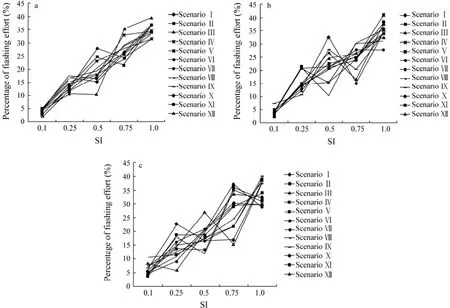
Fig.2 Percentages of fishing efforts in each value of SI for all the scenarios of different spatial scales with the temporal scale of (a) week, (b) fortnight, and (c) month.

For each temporal scale, the relationships between fishing effort and SI values among different scenarios are shown in Fig.2. The percentage of fishing effort varies for each SI value among different spatial scales. For weekly and biweekly scenarios, the largest difference of fishing effort occurs for SI value of 0.5 with the maximum and minimum values of 28.83% and 10.25% for weekly (Fig.2a), and 32.55% and 10.10% for biweekly (Fig.2b),respectively. The largest difference occurs for SI value of 0.75 with the maximum and minimum values of 37.17% and 15.19% for monthly scenarios (Fig.2c).

3.3 Overlay of Fishing Effort and SST Under Different Scales

To compare the impact of spatial scales of fisheries and SST data on evaluating and forecasting the distribution of fishing ground, we produced the maps of fishing efforts and SI values for SST with three different spatial scales (0.5˚ latitude and 0.5˚ longitude, 1˚ latitude and 1˚ longitude, 2˚ latitude and 2˚ longitude）when the temporal scale is fixed at fortnight in 2008 (Fig.3). The distribution of habitat and fishing efforts among different SI valuesshow large differences under three different spatial scales. The percentages of habitat area with more than 0.5 of SI are 41.39%, 28.89% and 50% when arranged from small spatial scale to large spatial scale, respectively, and the corresponding fishing efforts are 97.17%, 75.86% and 78.94% of the total (Fig.3).

Fig.3 Spatial distribution of the first biweekly total fishing days for Ommastrephes bartramii overlaid on the suitability index (SI) of sea surface temperature in the northwest Pacific Ocean from the Chinese Mainland Squid Technical Group in 2008 with different spatial scales of (a) 0.5˚ latitude and 0.5˚ longitude, (b) 1˚ latitude and 1˚ longitude, and (c) 2˚ latitude and 2˚ longitude.

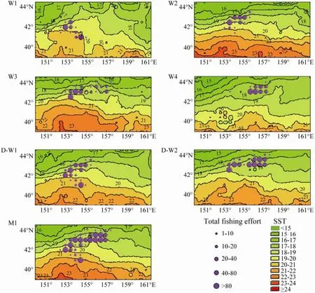
Fig.4 Spatial distribution of total fishing days for Ommastrephes bartramii overlaid on sea surface temperature (SST) in the northwest Pacific Ocean from the Chinese Mainland Squid Technical Group, 2008, with the fixed space of 0.5˚ latitude and 0.5˚ longitude, and different temporal scales from the first week to the fourth week (W1–W4), the first fortnight (D-W1) to the second fortnight (D-W2), and August (M1).

The fishing effort and SST data were aggregated with three different temporal scales when the spatial scale was fixed at 0.5˚ latitude and 0.5˚ longitude. The distribution of fishing effort and isotherm were mapped by different temporal scales, i.e., four weeks, two fortnight and one month at the beginning of August in 2008 (Fig.4). The spatial distribution of fishing effort shows obvious differences (Fig.4). The fishing ground is distributed in waters of 42˚N and west of 155˚E during the first week, began to move to the northeast in the second and third week, and aggregated mostly in 43˚N and the east of 155˚E in the fourth week (W1–W4; Fig.4). The change of fishing ground distribution might be found when the temporal scale was set as fortnight (D-W1 and D-W2; Fig.4). However, the difference is not obvious in monthly distribution, as the fishing ground is widely located in the waters of 41˚30´–43˚N and 152˚30´–157˚E (M1; Fig.4).

3.4 Comparing CVs in Different Scenarios

The CVs were calculated using Eq. (2) for weekly, biweekly and monthly SI under different spatial scales. The results are shown in Fig.5. For each scenario, CVs of SI rang from 0.51 to 0.63 for weekly data, from 0.52 to 0.73 for biweekly data, and from 0.47 to 0.71 for monthly data. To compare the impact of different latitude scales, the scenarios were divided into three groups based on latitude scales. The CVs tend to increase with the longitude scales and fluctuate little for all the scenarios in each temporal scale when the latitude scale was fixed (Fig.5a). The lowest CV was found when the longitude scale was set as 0.5˚ and the highest CV was obtained when the longitude scale was set as 2˚, except for the weekly scenario with the latitude scale of 1˚. When the longitude scales were fixed, the lowest CV was found at the latitude scale of 1˚ for weekly scenarios (Fig.6a). For biweekly data, the CVs tend to increase with latitude scale (Fig.6b). The same trend can be found for all monthly scenarios (Fig.6c).

3.5 Comparing Fishing Effort of Scenario I and Other Scenarios

The MRDI were calculated using Eq. (2) for other scenarios from the based spatial scale of 0.5˚ latitude and 0.5˚ longitude and were plotted for weekly (Fig.7a), biweekly (Fig.7b) and monthly total fishing effort (Fig.7c). MRDI values for weekly data increase quickly with the spatial scales, but the increase lessens when the spatial scale is larger than 2˚ squares (Fig.7a). The same trend could be found for month scenarios, but large MRDI values were found (Fig.7c). For the above two scenarios (Figs.7a and 7c), the relationship between MRDI and area of spatial grids can be described by the exponential function (P <0.05). While for biweekly data, MRDI values show much variation across the area of spatial grids (Fig.7b). The MRDI values increase when the size is smaller than 2˚ squares, and then decrease quickly and slowly increase from 4˚ squares to 8˚ squares (Fig.7b).

Fig.5 Coefficient of variation (CV) of the (a) weekly, (b) biweekly and (c) monthly SI values for all the scenarios with different longitude scales.

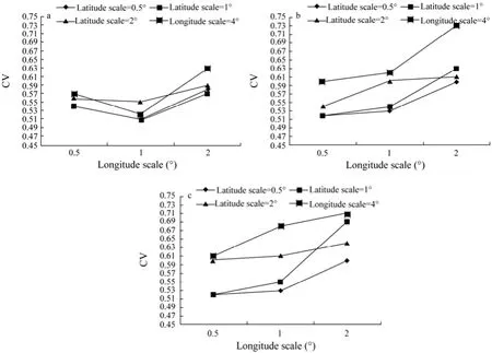
Fig.6 Coefficient of variation (CV) of the (a) weekly, (b) biweekly and (c) monthly SI values for all the scenarios with different latitude scales.

Fig.7 The mean relative variance (MRDI) calculated with Eq. (2) for (a) weekly, (b) biweekly and (c) monthly percentage of fishing effort with different spatial scales. The plotted lines described by an exponential function show the MRDI at different spatial scales. 1˚ latitude multiplied by 1˚ longitude means 1˚ area of spatial grid (1˚ square).

4 Discussion

Temporal scale is habitat lifespan relative to the generation time of the organism, and spatial scale is the distance between habitat patches relative to the dispersal distance of the organism (Fahrig, 1992). Thus, the choice of scales may greatly affect the evaluation of relationships between fisheries and biographical environmental variables (Perry and Ommar, 2003; Tian et al., 2009b). The distribution of fish population is likely to vary with space and time (Legendre and Fortin, 1989; Legendre, 1997). Generally the smaller scale we set on the data aggregation, the more precise will be the forecast of the HSI and fishing ground. However, financial costs are likely to increase greatly if we collect data in smaller scale. Therefore, we hope to identify an optimal cost-effective scale level that balances costs and precision of sampling. In this study,the environmental variable SST was used as an example to evaluate the effect of different scales on HSI, and we found that the optimal temporal and spatial scales with the lowest CV are month and 0.5˚ latitude and 0.5˚ longitude, respectively, for O. bartramii in the northwest Pacific Ocean. With the availability of ocean remote sensing data and improvement of data accuracy with different spatial and temporal scales, other environmental factors including sea surface height anomaly, SSS and Chl a need to be considered in future habitat modeling.

The distribution and migration of O. bartramii may be influenced by different marine environmental variables such as SST (Chen, 1997; Ichii et al., 2009). During different stages of life history, the preferred environmental variables may be different for O. bartramii in the northwest Pacific Ocean (Chen et al., 1997; Chen and Tian, 2005). Previous studies showed that there are different optimum SSTs for squid in different months and fishing areas, and there appear the tendency of optimum monthly SST gradually decreasing from west to east (Chen et al., 2008a).

The habitat model developed in this study is rather qualitative and may depend on scales we set for SI values. We found that the choices of SI values may influence the modeling results for different spatial and temporal resolutions. High quality habitat can provide high carrying capacity and support high rates of growth, survival, or reproduction of organisms. In this study, a simple HSI model only based on SST is used to show the effect of different spatial and temporal resolutions. However, the factors affecting squid habitat is complex. The impact of different variables on the HSI models for O. bratramii was studied and it was found that SST is the most important factor compared to the gradients of SST and SSH (Gong et al., 2012).

The large difference between percentages of fishing effort on each SI value suggests that the choice of spatial scale can have a great impact on weekly, biweekly or monthly habitat suitability modeling for O. bartramii based on the one environmental factor (SST). The CVs are different in each temporal scale when the spatial scale is different. This may result in the ecological and biological processes operating on different spatial and temporal scales. Previous results indicated that the distribution of O. bartramii is also determined by the food-rich subarctic front zone (SAFZ) and the transition zone (TZ) being located between the SAFZ and subtropical frontal zone (STFZ) (Ichii et al., 2009). Future studies including more environmental factors are needed in the habitat modeling of O. bartramii.

The CVs of SI values tend to increase along the longitude scale when the latitude scale is fixed for each temporal scale (Fig.5). When the longitude scale is fixed, the CVs of SI values tend to increase with the latitude scale for biweekly or monthly data, except for a little variation observed for weekly data. This could result from large SST variation between weeks, fortnights or months in both of the latitudinal and longitudinal directions (Chen and Tian, 2005; Chen et al., 2008a; Chen et al., 2010).

The variation of total percentage of fishing effort among SI values for monthly data that tended to increase quickly with the sizes of spatial square is larger than those for weekly or biweekly data (Fig.7). As a short life span species, neon flying squid moves fast, which allows it to migrate to the area with suitable SST (Chen et al., 2009). Therefore, the fishing ground may be different when the time interval is week. For weekly scenarios, the MRDI tends to increase with the size of area (Fig.7a). However, the difference is smaller than 10% when the area is limited as 1˚ square. That means if we allowed 10% of the average difference about fishing effort between the finest scale and the larger scale, the larger scale would be accepted for collecting and aggregating data.

The smallest scale is not always the best choice considering the CVs and research costs. It is desirable to identify cost-effective spatial and temporal scales for fishery data collection and analysis. However, different studies require different appropriate spatial and temporal scales of data collection. For example, some studies (Pitcher et al., 2000; Marrs et al., 2002) identified CPUE calculated by the ICES statistical rectangles (1˚×0.5˚), which makes it difficult to identify the fishery resource with higher productivity and limits its use as a reliable index of abundance. However, for longline tuna fisheries, 1˚ latitude × 0.5˚ longitude might be too small to reflect the dynamics of fishing effort because the length of longlines usually exceeds 1˚ (Tian et al., 2009b). Also, for a long life span and high migratory species such as sperm whales, the feeding success may vary with long time and large space (Whitehead, 1996). Therefore, larger spatial and temporal scales are needed for studying the habitat of sperm whales. It is recommended that if large scale data can yield the similar results to that at the small scale for fisheries, the large scale may be more appropriate in data collection and analysis (Tian et al., 2009b).

HSI model constructed from the single factor of SST can be applied to identify and evaluate potential fishing ground. Because of data limitation, we did not evaluate finer spatial and temporal scales. The SST data used in this paper were from remote sensing and we hope that the reflection of space and time of other environmental variables used to construct the HSI model could be improved. The habitat models with other environmental factors may further improve the forecasting of fishing area and each variable may have its own optimal scale. However, this study indicates that the choice of spatial and temporal scales in data collection and aggregation can significantly influence the fishery habitat modeling and the evaluation of fishery.

In summary, the objective of this study is to evaluate the roles of spatio-temporal scales in developing habitat suitability models using the western stock of winterspring cohort of O. bartramii in the northwest Pacific Ocean as an example. It is found that the optimal temporal and spatial scales with the lowest CV are month, and 0.5˚ latitude and 0.5˚ longitude for O. bartramii in the northwest Pacific Ocean. This study shows that temporal and spatial scales used for data aggregation can greatlyinfluence habitat suitability modeling. The habitat model developed with an optimal scale can improve the forecasting of fishing ground and favorable habitat.

Acknowledgements

We thank the Chinese Mainland Squid Technical Group for providing the fisheries data, and NASA for providing the SST data. This work was funded by National High Technology Research and Development Program of China (863 Program, 2012AA092303), Project of Shanghai Science and Technology Innovation (12231203900), Industrialization Program of National Development and Reform Commission (2159999), National Science and Technology Support Program (2013BAD13B01), and Shanghai Leading Academic Discipline Project. Also this study was supported by National Distant-Water Fisheries Engineering Research Center, and Scientific Observing and Experimental Station of Oceanic Fishery Resources, Ministry of Agriculture, P. R. China.

Andrade, H. A., and Garcia, A. E., 1999. Skipjack tuna in relation to sea surface temperature off the southern Brazilian coast. Fisheries Oceanography, 8: 245-254.

Bower, J. R., and Ichii, T., 2005. The red flying squid (Ommastrephes bartramii): A review of recent research and the fishery in Japan. Fisheries Research, 76: 39-55.

Brooks, R. P., 1997. Improving habitat suitability index models. Wildlife Soc B, 25: 163-167.

Brown, S. K., Buja, K. R., Jury, S. H., Monaco, M. E., and Banner, A., 2000. Habitat suitability index models for eight fish and invertebrate species in Casco and Sheepscot Bays, Maine. North American Journal of Fisheries Management, 20: 408-435.

Callicott, J. B., 2002. Choosing appropriate temporal and spatial scales for ecological restoration. Journal of Bioscience, 27: 409-420.

Cao, J., Chen, X. J., and Chen, Y., 2009. Influence of surface oceanographic variability on abundance of the western winter-spring cohort of neon flying squid Ommastrephes bartramii in the NW Pacific Ocean. Marine Ecology Progress Series, 381: 119-127.

Chen, X. J., 1997. An analysis on marine environment factors of fishing ground of Ommastrephes bartramii in northwest Pacific. Journal of Shanghai Fisheries University, 6: 285-287 (in Chinese).

Chen, X. J., and Tian, S. Q., 2005. Study on the catch distribution and relationship between fishing grounds and surface temperature for Ommastrephes bartramii in the northwestern Pacific Ocean. Periodical of Ocean University of China, 35: 101-107 (in Chinese with English abstract).

Chen, X. J., Zhao, X. H., and Chen, Y., 2007. Influence of El Niño/La Niña on the western winter-spring cohort of neon flying squid (Ommastrephes bartramii) in the northwestern Pacific Ocean. ICES Journal of Marine Science, 64: 1152-1160.

Chen, X. J., Chen, Y., Tian, S. Q., Liu, B. L., and Qian, W. G., 2008a. An assessment of the west winter-spring cohort of neon flying squid (Ommastrephes bartramii) in the Northwest Pacific Ocean. Fisheries Research, 92: 221-230.

Chen, X. J., Liu, B. L., and Chen, Y., 2008b. A review of the development of Chinese distant-water squid jigging fisheries. Fisheries Research, 89: 211-221.

Chen, X. J., Liu, B. L., and Wang, Y. G., 2009. Cephalopods in the World. Ocean Press, Beijing, 298pp.

Chen, X. J., Tian, S. Q., Chen, Y., and Liu, B. L., 2010. A modeling approach to identify optimal habitat and suitable fishing grounds for neon flying squid (Ommastrephes bartramii) in the Northwest Pacific Ocean. Fishery Bulletin, 108: 1-14.

Fahrig, L., 1992. Relative importance of spatial and temporal scales in a patchy environment. Theoretical Population Biology, 41 (3): 300-314.

Gillenwater, D., Granata, T., and Zika, U., 2006. GIS-based modeling of spawning habitat suitability for walleye in the Sandusky River, Ohio, and implications for dam removal and river restoration. Ecological Engineering, 28: 311-323.

Gómez, S., Menni, R., Naya, J., and Ramirez, L., 2007. The physical-chemical habitat of the Buenos Aires pejerrey, Odontesthes bonariensis (Teleostei, Atherinopsidae), with a proposal of a water quality index. Environmental Biology of Fishes, 78: 161-171.

Gong, C. X., Chen, X. J., Gao, F., and Chen, Y., 2012. Importance of weighting for multi-variable habitat suitability index model: A case study of winter-spring cohort of Ommastrephes bartramii in the Northwestern Pacific Ocean. Journal of Ocean University of China, 11: 241-248.

Gore, J. A., and Bryant, R. M., 1990. Temporal shifts in physical habitat of the crayfish, Orconectes neglectus (Faxon). Hydrobiologia, 199: 131-142.

Ichii, T., Mahapatra, K., Sakai, M., and Okada, Y., 2009. Life history of the neon flying squid: Effect of the oceanographic regime in the North Pacific Ocean. Marine Ecology Progress Series, 378: 1-11.

Zhang, D. E. (adaper), 2005. Miller and Freund’s Probability of Statistics for Engineers. 7th edition, Publishing House of Electronics Industry, Beijing, 569pp.

Legendre, L., and Fortin, M. J., 1989. Spatial pattern and ecological analysis. Plant Ecology, 80: 107-138.

Legendre, P., Thrush, S. F., Cummings, V. J., Dayton, P. K., Grant, J., Hewitt, J. E., Hines, A. H., McArdle, B. H., Pridmore, R. D., Schneider, D. C., Turner, S. J., Whitlatch, R. B., and Wilkinson, M. R., 1997. Spatial structure of bivalves in a sandflat: Scale and generating processes. Journal of Experimental Marine Biology and Ecology, 216: 99-128.

Levin, S. A., 1992. The problem of pattern and scale in ecology. Ecology, 73: 1943-1967.

Marceau, D. J., and Hay, G. J., 1999. Remote sensing contributions to the scale issue. Canadian Journal of Remote Sensing, 25: 357-366.

Marrs, S. J., Tuck, I. D., Atkinson, R. J. A., Stevenson, T. D. I., and Hall, C., 2002. Position data loggers and logbooks as tools in fisheries research: Results of a pilot study and some recommendations. Fisheries Research, 58 (1): 109-117.

Morrison, M. L., Marcot, B. C., and Mannan, R. W., 1998. Wildlife-Habitat Relationship: Concepts and Applications. University of Wisconsin Press, Madison, 416pp.

National Research Council, 1982. Impacts of emerging agricultural trends on fish and wildlife habitats. National Academy, Washington D C.

Perry, R. I., and Ommer, R. E., 2003. Scale issues in marine ecosystems and human interactions. Fisheries Oceanography, 12: 513-522.

Pitcher, C. R., Poiner, I. R., Hill, B. J., and Burridge, C. Y., 2000. Implications of the effects of trawling on sessile megazooben-thos on a tropical shelf in north-eastern Australia. ICES Journal of Marine Science, 57: 1359-1368.

Schwartz, M. L., 2005. Encyclopedia of Costal Science. Springer Press, Netherlands, 194pp.

Swain, D. P., Wade, E. J., 2003. Spatial distribution of catch and effort in a fishery for snow crab (Chionoecetes opilio): Tests of predictions of the ideal free distribution. Canadian Journal of Fisheries and Aquatic Sciences, 60: 897-909.

Tian, S. Q., Chen, X. J., Chen, Y., Xu, L. X., and Dai, X. J., 2009a. Evaluating habitat suitability indices derived from CPUE and fishing effort data for Ommatrephes bartramii in the northwestern Pacific Ocean. Fisheries Research, 95: 181-188.

Tian, S. Q., Chen, Y., Chen, X. J., Xu, L. X., and Dai, X. J., 2009b. Impacts of spatial scales of fisheries and environmental data on catch per unit effort standardization. Marine and Freshwater Research, 60: 1273-1284.

Tomsic, C. A., Granata, T. C., Murphy, R. P., and Livchak, C. J., 2007. Using a coupled eco-hydrodynamic model to predict habitat for target species following dam removal. Ecological Engineering, 30: 215-230.

U. S. Fish and Wildlife Service, 1981. Standards for the development of habitat suitability index models. U S Fish and Wildlife Service 103 ESM: 1-81.

Van der Lee, G. E. M., Van der Molen, D. T., Van der Boogaard, H. F. P., and Van der Klis, H., 2006. Uncertainty analysis of a spatial habitat suitability model and implications for ecological management of water bodies. Landscape Ecology, 21: 1019-1032.

Vinagre, C., Fonseca, V., Cabral, H., and Costa, M. J., 2006. Habitat suitability index models for the juvenile soles, Solea solea and Solea senegalensis, in the Tagus estuary: Defining variables for species management. Fisheries Research, 82: 140-149.

Vincenzi, S., Caramori, G., Rossi, R., and Leo, G. A. D., 2006. A GIS-based habitat suitability model for commercial yield estimation of Tapes philippinarum in a Mediterranean coastal lagoon (Sacca di Goro, Italy). Ecological Modelling, 193: 90-104.

Whitehead, H., 1996. Variation in the feeding success of sperm whales: temporal scale, spatial scale and relationship to migrations. Journal of Animal Ecology, 65: 429-438.

Wang, Y. G., and Chen, X. J., 2005. The resource and biology of economic oceanic squid in the world. Ocean Press, Beijing, 366pp.

Yatsu, A., Midorikawa, S., Shimada, T., and Uozumi, Y., 1997. Age and growth of the neon flying squid, Ommastrephes bartramii, in the North Pacific Ocean. Fisheries Research, 29: 257-270.

Zainuddin, M., Kiyofuji, H., Saitoh, K., and Saitoh, S. I., 2006. Using multi-sensor satellite remote sensing and catch data to detect ocean hot spots for albacore (Thunnus alalunga) in the northwestern North Pacific. Deep Sea Research II: 53: 419-431.

(Edited by Qiu Yantao)

(Received March 1, 2013; revised April 15, 2013; accepted May 13, 2014)

© Ocean University of China, Science Press and Spring-Verlag Berlin Heidelberg 2014

* Corresponding author. Tel: 0086-21-61900306

E-mail: xjchen@shou.edu.cn