Interpurchase Time of Customer Behavior in Cloud Computing

Hui-Hsin Huang

1. Introduction

Cloud computing is a more and more popular paradigm for accessing computing resources, which are delivered as a service over a network[1]. As cloud computing is applying in marketing, the managers can collect data of customer purchase behavior from cloud platforms and use database as a service (DBaaS), which is one of public cloud computing types to predict the customer purchase pattern, such as interpurchase time.The interpurchase time is the duration or spell between two consecutive purchases. The measurement of customer interpurchase time is important because it indicates the customer attractiveness[2]. The customers who interact frequently with a firm are viewed as being more satisfied with their transactions and represent a more important stream of income than those who interact infrequently[3]. For a firm, interpurchase time is used as a metric in evaluating decisions in the context of customer value management[4]. Accordingly, marketing researchers have developed a number of models to discuss this topic. This paper perceives interpurchase time as an dynamic process and propose a stochastic model to describe customer’s interpurchase behavior.

2. Literature Review

Many marketing researchers have developed a number of models to discuss the interpurchase time topic. Some of them proposed statistical distributions, such as Erlang-2 and negative binomial[5], and used panel data to estimate parameters of purchase-timing[6]. Some used econometric models, such as the logistic regression model, to deal with the effects of marketing variables[7]which influence purchase timing decision. Accordingly, these models are kinds of continuous models which assume that interpurchase interval is a continuous variable.

Some models considered time intervals of purchase as discrete[4],[8]. Borle et al.[8]measured interpurchase time in weeks and assumed that it followed a negative binominal distribution (NBD) which was a well known and used distribution in marketing literature. It is a generalization of the Possoin distribution and is useful in modeling over dispersed count data. Boatwright et al.[4]used Conway-Maxwell-Possion (CM-Poisson) to model the week of next purchase. Their models correspond to interdelivery time that was multiples of 7 days, indicating that there was a strong tendency for customers to request deliveries in intervals of a week. In part, the weekly tendency could correspond to the planning and purchase schedule of the individual households, which might plan the meals and household inventory on a weekly basis.

However, these models only pay attention on depicting interpurchase time to suppose it as a continuous or discrete form. But in the competitive marketing environment,customers may behave multi-brand choices and demonstrate multi-brand loyalty[9]-[12]. For a signal brand(product), the interpurchase time of its customer is not always stable. When this customer transacts with other brands, his interpurchase time of this brand will become increase. On the contrary, if he is sticky with this brand and makes more transactions, then his interpurchase time of this brand will become decrease. Previous researches did not develop a model to capture this changing and dynamic process. This paper bases on this trend to reconstruct an interpurchase model.

3. Interpurchase Model

We consider that the lifetime of the interpurchase time to a customer is followed a geometric pattern. In the long-term trend, the empirical data of interval time of transactions will first decrease then increase. The scenario of the decreasing is captured that the customer will be more familiar with this brand after a few times of purchase and purchase it as the primary brand (or loyal brand) of this product category on his usual shopping list. After a period of time, the customer will no more be loyal to this brand thus the interpurchase time will decrease until he defects from this brand.

Our model can be decomposed into two components:one is that the baseline of interpurchase time which is denoted as W1, W2, ⋅⋅, Wnand follows an exponential density function; the other is that the geometric parameters ciand hicapture the trend of the dynamic process that the interpurchase time decreases before a point of time and increases after this time point. We call this point of time as the “change point”. In this section, we first demonstrate the full geometric model. Then, the difference of the geometric parameters before and after the change point will be introduced.

3.1 Interpurchase Time Model

The ith interpurchase time is denoted as xiwhich follows the geometric density function as

where()I⋅is the indicator function, i is the ith interpurchase time and τ is the change point of the interpurchase time, Wiis the base line in the exponential form of λe-λx, and ciand hiare the geometric parameters.

Thus, we consider the interpurchase time x before the change point as

f (x c, i) = ciλ e x p (- ciλ x ) (2)
before

and interpurchase time x after the change point is

A. Before Change Point

We consider the parameter c following the uniform distribution between 0 and 1, that is, c ～ U(0,1)

Then, the probability of density function of interpurchase time before the change point is

where

B. After Change Point

We consider the parameter h following the uniform distribution between 1 and q: ),1(～qUh

Then, the marginal density of interpurchase time after the change point is

Finally, we can obtain the marginal density of (1) by(5) plus (7).

4. Change Point

In this section, we discuss the parameters of the change point. We assume that a customer starts to change his pattern of purchasing after random transactions. Then his interpurchase time interval may vary from decreasing to increasing with the change point τ. Therefore, the change point, at which the customer changes his purchasing behavior, is distributed across transactions.

Then, we consider two discrete models: Bernoulli and Poisson processes.

4.1 Bernoulli Process of Change Point

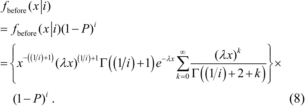
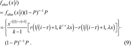
When assuming that the distribution of the change point follows the Bernoulli process with a parameter P, we can develop the marginal density of interpurchase time in the Bernoulli process to the change point according to (5) and(7).

Based on (5), the marginal density of the interpurchase time before the change point is

Based on (7), the marginal density of the interpurchase time after the change point is

4.2 Poisson Process of Change Point

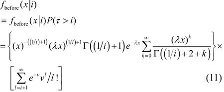
If we consider the change point following the Poisson process with a parameterv: τ ～Possion(v), then, we can calculate the probability of the change point τ=l as follows:

Based on (5) and (7), we can obtain the marginal density of interpurchase time in the Poisson process to the change point.

According to (5) and (10), if the change point is after the ith transaction, the marginal density of interpurchase time before the change point can be demonstrated as

If the change point is j which is before the ith transaction, (12) can be obtained by (7) and (10).

5. Conclusions

In this paper, we consider a dynamic process of interpurchase time. Because the distribution of interpurchase time is generally influenced by marketing variables and customer characteristics, customers’ life cycles are becoming increasing due to the impact of competitors actions on existing relationships[13]. The geometric distribution will be more effective for reflecting the variety purchase interval which may not be at a steady rate. It is also more applicable to cloud computing especially to online shopping. Customers will be easier to be variety-seeking in online shopping which supplies various brands and provides many choices for purchase.Thus a customer may purchase multi-brands at the same time and demonstrate multi-loyalty. Accordingly, the concept of change point can characterize that the customer may still purchase the same brand but the frequency of transactions is dynamic, and the interpurchase time shows different trends before and after the change point. (the interpurchase time is decreasing before the change point and increasing after the point).

The contribution of this paper is to provide a geometric point of view (instead of signal probability distribution function) to model interpuchse time. In the future, we can consider different kinds of distribution to descript the change point and geometric process.

[1] S. Bhardwaj, L. Jain, and S. Jain, “Cloud computing: a study of infrastructure as a service (IAAS),” Int. Journal of Engineering and Information Technology, vol. 2, no. 1, pp.60-63, 2010.

[2] D. Fok, R. Paap, and P. H. Franses, “Modeling dynamic effects of promotion on interpurchase times,”Computational Statistics & Data Analysis, vol. 56, no. 11,pp. 3055-3069, 2012.

[3] D.-S. Dong and K. M. Harry, “Investigating coupon effects on household interpurchase behavior for cheese,” in Proc. of American Agricultural Economics Assosiation Annual Meeting, Long Beach, 2006, pp. 23-26.

[4] P. Boatwright, S. Borle, and J. B. Kadane, “A model of the joint distribution of purchase quantity and timing,” Journal of the American Statistical Association, vol. 98, no. 463, pp.564-572, 2003.

[5] B. P. Seetharaman and P. K. Chintagunta, “The proportional hazard model for purchase timing: a comparison of alternative specifications,” Journal of Business and Economic Statistics, vol. 21, no. 3, pp. 1-15, 2002.

[6] C. Chatfield and G. J. Goodhardt, “A consumer purchasing model with erlang inter-purchase times,” Journal of the American Statistical Association,” vol. 68, no. 344, pp.828-835, 1973.

[7] P. B. Seetharaman, “The additive risk model for purchase timing,” Marketing Science, vol. 23, no. 2, pp. 234-242,2004.

[8] S. Borle, S. S. Singh, and J. C. Dipak, “Customer lifetime value measurement,” Management Science, vol. 54, no. 1,pp. 100-112, Jan. 2008.

[9] C. Homburg and A. Gierin, “Personal characteristics as moderators of the relationship between customer satisfaction and loyalty—an empirical analysis,” Psychology and Marketing, vol. 18, no. 1, pp. 43-66, 2001.

[10] H. A. Roehm Jr. and M. L. Roehm, “Revisiting the effect of positive mood on variety seeking,” Journal of Consumer Research, vol. 32, no. 2, pp. 330-336, 2005.

[11] J. Choi, B. K. Kim, I. Choi, and Y. Yi, “Variety-seeking tendency in choice for others: interpersonal and intrapersonal causes,” Journal of Consumer Research, vol.32, no. 4, pp. 590-595, 2006.

[12] C. Goukens, S. Dewitte, M. Pandelaere, and L. Warlop,“Wanting a bit(e) of everything: extending the valuation effect to variety seeking,” Journal of Consumer Research,vol. 34, no. 3, pp. 386-394, 2007.

[13] W. J. Reinartz and V. Kumar, “On the profitability of long-life customers in a noncontractual setting: an empirical investigation and implications for marketing,” Journal of Marketing, vol. 64, no. 4, pp. 17-35, 2000.