Stochastic simulation of fluid flow in porous media by the complex variable expression method*

SONG Hui-bin (宋会彬), ZHAN Mei-li (詹美礼), SHENG Jin-chang (盛金昌), LUO Yu-long (罗玉龙)

College of Water Conservancy and Hydropower Engineering, Hohai University, Nanjing 210098, China, E-mail: shbsgf@163.com

Stochastic simulation of fluid flow in porous media by the complex variable expression method*

SONG Hui-bin (宋会彬), ZHAN Mei-li (詹美礼), SHENG Jin-chang (盛金昌), LUO Yu-long (罗玉龙)

College of Water Conservancy and Hydropower Engineering, Hohai University, Nanjing 210098, China, E-mail: shbsgf@163.com

(Received March 28, 2012, Revised January 18, 2013)

A stochastic simulation of fluid flow in porous media using a complex variable expression method (SFCM) is presented in this paper. Hydraulic conductivity is considered as a random variable and is then expressed in complex variable form, the real part of which is a deterministic value and the imaginary part is a variable value. The stochastic seepage flow is simulated with the SFCM and is compared with the results calculated with the Monte Carlo stochastic finite element method. In using the Monte Carlo method to simulate the stochastic seepage flow field, the hydraulic conductivity is assumed in three different probability distributions using random sampling method. The obtained seepage flow field is examined through skewness analysis, and the skewed distribution probability density function is given. The head mode value and the head comprehensive standard deviation are used to represent the statistics of calculation results obtained by the Monte Carlo method. The stochastic seepage flow field simulated by the SFCM is confirmed to be similar to that given by the Monte Carlo method from numerical aspects. The range of coefficient of variation of hydraulic conductivity in SFCM is larger than used previously in stochastic seepage flow field simulations, and the computation time is short. The results proved that the SFCM is a convenient calculating method for solving the complex problems.

seepage flow field, complex variable expression method (SFCM), stochastic seepage flow, Monte Carlo method, skewed distribution

Introduction

Hydraulic conductivity is an important parameter in seepage flow analysis. In the traditional seepage flow analysis, the variability of hydraulic conductivity parameter has not been considered and therefore the results could not reflect practical conditions. With advances in understanding the theory of reliability in recent years, more attention has been paid in conducting uncertainty analysis in engineering design and numerical analysis. Dogan and Motz[1]pointed out that the main reason leading to the random nature of the seepage field is the randomness of the hydraulic conductivity parameter. Fiori and Dagan[2]modeled hydraulic conductivity as a stationary random space function and researched the transport of a passive scalar in a stratified porous medium. Zhang et al.[3-5]carried out a systematic study of random model of unsaturated steady seepage and unsteady seepage. Amir and Neuman[6,7]proposed a Gaussian closure approximation for steady state and transient unsaturated flow problems in randomly heterogeneous soils. Yang et al.[8]used the random numerical method which combined the Karhunen Loeve expansion and perturbation method together for analyzing saturated-unsaturated seepage problems. Li et al.[9]discussed the random characteristics of porous medium permeability coefficient through combining the First-Order Reliability Method (FORM) with the Lattice Boltzmann Method (LBM). Wang et al.[10]used the Monte Carlo method to study the three-dimensional stochastic seepage field of the Yangtze River embankment in the complex boundary conditions with prevention measures. The Monte Carlo method, which is usually used to analyze stochastic seepage flow field, requires a lot of random sampling data and the statistical characteristics of seepage flow field can be obtained through multiple repeated calculation of the certainty of seepage flow.This method, because of easy-to-calculation and potential to have high accuracy, is referred to be a good seepage flow simulation method. The mean value of head is used to represent the statistic of calculation result that obtained by the Monte Carlo method in stochastic seepage flow simulation. The data with the highest frequency is of the main concern in engineering practice. The results calculated with the Monte Carlo method often obey a skewed distribution. While for the single-peak asymmetric probability distribution, the mean value and mode value are not equal (note that the mode is defined as the marker value with the most appearing times in general, or the variable with the highest times in a variable series[11]). So the theoretical results and the required values of practical engineering application are slightly different.

Because of large number of sampling and large amount of calculations needed when using the Monte Carlo method, it is restricted in practical engineering applications. Many scholars used the finite element method for studies of stochastic seepage flow, and obtained encouraging results. For example, Sheng et al.[12]introduced the first-order Taylor series to analyze the stochastic relationship between permeability of jointed rock masses and basic geometric parameters of joints using a model of equivalent continuous medium. Li et al.[13]inferred the three-dimensional steady seepage flow stochastic finite element formulistic, which was applied to stochastic seepage flow calculation. Wang et al.[14]derived the stochastic finite element formulation of three-dimensional unsteady seepage flow, which was combined with the firstorder Taylor series expansion of the stochastic FEM to derive a formula for calculating the mean and variance of flow in the seepage flow field. This method considered that the maximum coefficient of variation of hydraulic conductivity is 0.3 of the porous medium. And the variation range of coefficient of hydraulic conductivity here had some discrepancy with the practical engineering. Based on the shortcomings of above methods, the complex issue of the large variability seepage flow calculation problem is considered in this article. A new stochastic simulation method of fluid flow in porous media is provided, which is named seepage flow field, complex variable expression method (SFCM). In this method, the hydraulic conductivity is expressed in complex variable form, with its real part being a deterministic value and its imaginary part being a variable value. The complex variable form expression is calculated using a selfcompiling program solving linear equations with complex coefficients based on the finite element method. The results calculated with the Monte Carlo method showed a skewed distribution, and the mode is used to represent its statistics. The skewed distribution probability density function and the method to calculate standard deviation are provided in this article. Finally the relationship of stochastic seepage flow field simulated by the Monte Carlo method and SFCM is discussed in the numerical aspects with the hydraulic conductivity of different probability distributions and coefficients of variation. The results show that the SFCM is featured by simple calculation, small amount of calculation, and large-range variation of parameters.

1. Resolution method with complex variable expression

In practice, the hydraulic conductivity of porous medium is determined using laboratory tests on several samples obtained from field. So the hydraulic conductivities of natural rock mediums all show some discreteness. Engineers usually calculate the mean value and standard deviation for researchers for simulation. Not only the results of the seepage flow analysis using the mean value but also the corresponding distributions of seepage flow calculated with the standard deviation value should be concerned in the engineering design. Generally, two methods were used in the past to analyze seepage flow field variation: (1) the Monte Carlo method, through statistical analysis of a lot of seepage flow simulation results, giving the mean value and variance of seepage flow field, (2) the Taylor expansion method, expressing the calculation result of governing equation as the second order Taylor expansion in the mean value of hydraulic conductivity, and giving then the mean value and variance. The former is hard to implement with large amount of calculations for large complex problems. The latter is applied only to smaller variation range of parameters, and often difficult to get convergence when the parameter variation is slightly larger. A new resolution method with complex variable expression is presented in this article to overcome the defects of the above methods and improve the original expression of the parameter variation.

The expression of random hydraulic conductivity is similar to the instantaneous velocity expression mode typically used in fluid mechanics. The expression of instantaneous velocity is given as

The expression of random hydraulic conductivity is similar to Eq.(1) and is shown as

wherek is random hydraulic conductivity,is the mean of hydraulic conductivity,k˜is the deviation of random hydraulic conductivity, which are all realnumbers.µis the mean value of hydraulic conductivity, andσis the standard deviation of hydraulic conductivity and is nonnegative. So Eq.(2) can be rewritten as follows when it is used to express the statistics of hydraulic conductivity

Based on Eq.(3) we use complex variable to replace it to distinguish the respective position between mean value and standard deviation. Then the hydraulic conductivity is expressed as follows

where iis the imaginary unit. In Eq.(4), it is clearly shown that the two statistic values of hydraulic conductivity can be well expressed in complex variable form. The remarkable advantage of this expression is that the complex variable calculation result can be directly obtained by solving the governing equations of seepage flow with hydraulic conductivity expressed in complex variable form.

2. Stochastic analysis of seepage flow with hydraulic conductivity expressed in complex variable form

The differential equation of three-dimensional steady seepage flow[15]is as follows

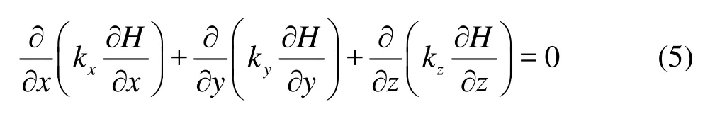
where kx,ky,kzare the orthotropic hydraulic conductivities. The finite element formulation of Eq.(5) is

where K is the hydraulic conductivity matrix,H and F are the hydraulic head column vectorsand the equivalent flowcolumn vectors, respectively, for the seepage flow field. The hydraulic conductivity in the matrixKis considered as a random variable, and expressed in complex variable form as follows

where the real part k is the mean value of hydraulic conductivity. It is the deterministic component, and the steady seepage flow field can be obtained by using it in seepage flow calculation.αis the coefficient of variation of hydraulic conductivity. The variation of hydraulic conductivity can be obtained by multiplying αandk , namely the standard deviation or comprehensive standard deviation. It is the variable component, and thus the variable amplitude of the steady seepage flow field can be calculated. The essence of Eq.(4) and Eq.(7) is the same although the representa

regarded as tion is slightly different. The hydraulic conductivity, which is expressed in form of Eq.(7), is just a simple complex variable and it does not involve complex analytic function. Head and flux boundary conditions are taken into account in Eq.(6), and they are

certainty conditions with no variation. Although they can be expressed in the complex variable form, their imaginary parts are zero.

Fig.1 Flowchart of seepage flow calculation program

The stochastic seepage flow field can be calculated by a self-compiling program solving linear equations with complex coefficients based on the finite element method. Water head is expressed in complex variable form as followswhereH is the head,His the head variation. The head variation, which is caused by variable amplitude value of hydraulic conductivity, is the head offset value. It is also another sense of standard deviation. Therefore the head variation values are all taken absolute values. The stochastic seepage flow field, which is simulated by the SFCM, can be obtained through the calculation process as shown in Fig.1.

In order to confirm the correctness and feasibility of SFCM, the authors compare it with Monte Carlo method in stochastic seepage flow field simulation. The relationship of the SFCM and the Monte Carlo method has not been documented in literature. This paper addresses this relationship.

3. Skewed distribution

Wang et al.[10]considered hydraulic conductivity tensor k of seepage flow field as an independent random variable with the normal distribution. Hu et al.[16]presented hydraulic conductivity of roller compacted concrete which showed the logarithmic normal distribution through indoor experimentation and analysis. But the statistical results showed that the head values calculated with the Monte Carlo method are in skewed distribution, no matter whether the hydraulic conductivity is in the normal distribution or the logarithmic normal distribution. The data with the highest frequency, namely mode, receives the most concern in engineering practice. The mean value and mode are not equal for single-peak asymmetric probability distribution. So the mode is used as the representative value of calculation results with the Monte Carlo method in this article.

The results calculated with the Monte Carlo method are used in skewness analysis, and the skewed distribution probability density function is determined as follows

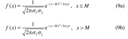
where M is the mode,1σis the left standard deviation (statistical standard deviation ofx≤M),2σis the right standard deviation (statistical standard deviation ofx＞M ). It is known from the definition of density function that

Comprehensive standard deviationσcan be obtained by the integration of Eq.(9). The expression of comprehensive standard deviationσis as follows

The comprehensive standard deviation is smaller than the traditional standard deviation in skewed distribution, and it reflects the comprehensive discrete degree of data. The offset influence of data, whether it is too large or too little, is effectively reduced. When σ1＜σ2, Eq.(9) shows that the data are shifted to the left, namely positive skewed distribution. And correspondingly when σ1＞σ2, Eq.(9) shows that the data are shifted to the right, namely negative skewed distribution. For the single-peak symmetric probability distribution such as uniform distribution and normal distribution, the mean value µ and mode M are equal. So whenσ1=σ2, Eq. can be simplified to normal distribution probability density function as follows

In order to better meet the field conditions, the mode and comprehensive standard deviation are used as the representative values of statistic calculated with the Monte Carlo method in stochastic seepage flow simulation in this article.

4. Random sampling

In the Monte Carlo method for stochastic seepage flow simulation, the hydraulic conductivity with a certain probability distribution should be assumed first, and random sampling is made according to the selected distribution. Mathematical methods, which are mainly used in computer, physical methods and random number tables are usually the methods used for generating random numbers. Pseudo random numbers can be produced using many mathematical methods, such as the Middle-Square method, the congruence method, etc.. In order to compare the stochastic seepage flow fields simulated by the Monte Carlo method and SFCM, the hydraulic conductivities in three different probability distributions are developed. They are the uniform distribution, normal distribution and skewed distribution. The procedure of extracting random number is as follows:

Step (1): Select the size of sampleN.

Step (2): Select the sample interval of extracting the random numbers X1to X2, then calculate the mean of sample µ.

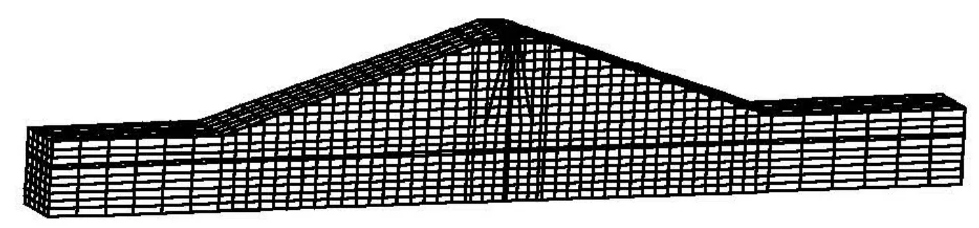
Fig.2 Finite element grid of earth-rock dam

Fig.3 Section plane of earth-rock dam

Step (3): Determine the main parameters of the three probability distributions: (a) the normal distribution: according to3σprinciple, calculate the sample standard deviation σ, (b) the skewed distribution: based on the principle of the sample tend to logarithmic normal distribution, work out parameters as the mode M, the left standard deviation1σand the right standard deviation2σthrough debugging the parameters in Eq.(9).

Step (4): Divide the sample interval, uniform distribution and normal distribution: evenly divide the sample interval into n, skewed distribution: divide the sample interval into n1and n2on both sides of mode M.

Step (5): Divide different interval numbers according to different probability distributions, work out the mean value and the corresponding frequency fiof each subinterval.

Step (6): According to the frequency fiand the size of sampleN , work out the frequency number nAof each subinterval.

Step (7): Use the congruence method to generate random numbers of uniform distribution in the corresponding frequency number nAof each subinterval.

Step (8): Fit the sample data of extraction, and work out the main parameters of the corresponding probability distribution: mean µ, standard deviation σ, or mode M left standard deviation1σ, right standard deviation2σ. Calculate the comprehensive standard deviation σby Eq.(11) when fitting function is skewed distribution.

The independence of each random number is perfectly guaranteed by the above method, and the uniformity is also well achieved. The random sampling of hydraulic conductivity is in uniform distribution, normal distribution and skewed distribution when the Monte Carlo method is used to simulate the stochastic seepage flow field. The relationship of the modes in different probability distributions in the same range of random sample data is as follows: skewed distribution < normal distribution = uniform distribution, the relationship of the comprehensive standard deviation is: skewed distribution < normal distribution < uniform distribution.

The most common method of generating the random number from 0 to 1 is the congruence method. Defined as if the remainders of two integers a and b , which divided by a positive integerm , are equal, then a and b are called the m congruence. The random numbers of other probability distribution can be obtained by changing the random numbers of uniform distribution from 0 to 1. The random numbers of each subinterval are generated by the congruence method.

The probability density function of uniform distribution is defined as

Obviously its range R is from 0 to 1, and the random variables of uniform distribution can be obtained according to the pseudo random number from 0 to 1 asfollows

5. Numerical varfication

Seepage flow under an earth-rock dam on pervious foundation is analyzed in this article. The finite element model is shown in Fig.2, and the subsurface stratigraphy is in Fig.3. The upstream water level elevation of the earth-rock dam is 52 m, the downstream water level elevation is 28 m, the depth of earth-rock dam curtain is 8 m, and the width of the calculation dam section is 20 m. The hydraulic conductivity of each media shown in Table 1.

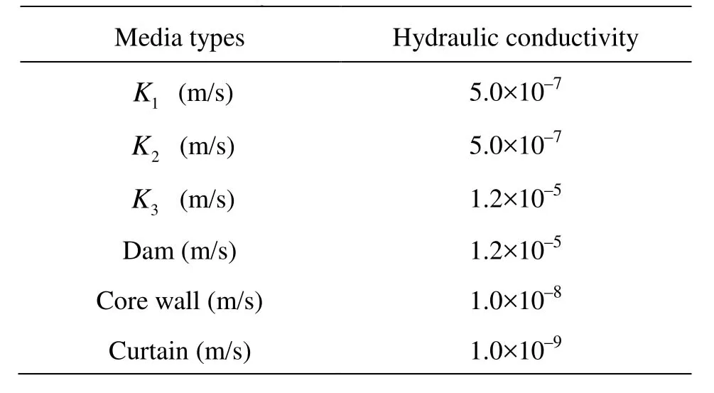
Table 1 Statistics of hydraulic conductivities

The hydraulic conductivities of medium are assumed to be the same in the three directions in this example. And the variation of curtain hydraulic conductivity is only considered in this article. The curtain hydraulic conductivity ranges from 1.4×105m/s to 1.4×10–7m/s as calculated using the Monte Carlo method. Three different kinds of probability distributions as described in the previous section are used for random sampling of the hydraulic conductivity. Five groups are randomly selected in each probability distribution within the range of hydraulic conductivity, and 1 500 random numbers were chosen within each group. Because of the difference between random numbers for different groups, the fitting comprehensive standard deviation is also different. The coefficient of variation of hydraulic conductivity is the ratio of the comprehensive standard deviation and corresponding mode in each group. The relationship of coefficients of variation in three different probability distributions is: skewed distribution > uniform distribution > normal distribution. The comprehensive standard deviation of skewed distribution is the smallest, and its mode is also the smallest, but the corresponding coefficient of variation is the largest. In order to compare the results from this article with those presented in the literature, the coefficient of variation is used to distinguish the computational results with different kinds of probability distributions in the following discussion. The range of coefficient of variation for sample data in this article is 0.32 to 0.71. When the stochastic seepage flow field is simulated by SFCM, the real part of curtain hydraulic conductivity is the mode and the imaginary part is the comprehensive standard deviation of sample data in each group.

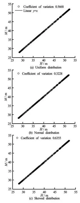
Fig.4 Comparison of head and head mode for three different kinds of probability distributions

5.1 Validation of SFCM

The node head and head variation obtained with the SFCM are compared in this section with those calculated using the Monte Carlo method in three different kinds of probability distributions. (The node head and head variation obtained with the SFCM are referred to as “head and head variation” in the following discussion). The relationships between the head obtained using the SFCM and head mode calculated using the Monte Carlo method are shown in Fig.4. The nodes shown in Fig.4 are all under the saturation linein the selected section. The best fitting linear regression line for the data is also shown in Fig.4, which indicates a strong fitting for the data with slope of the relationship at 1.0.

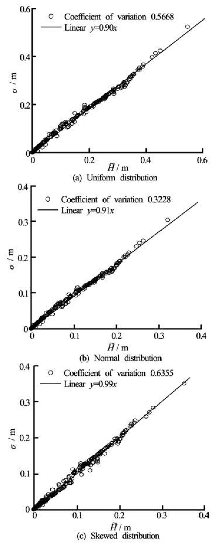
Fig.5 Comparison of head variation value and head comprehensive standard deviation in the three different kinds of probability distributions

The relationships between the head variation values obtained by the SFCM and the head comprehensive standard deviation values calculated by Monte Carlo method are shown in Fig.5.

The best fitting linear regression lines for the data is also shown in Fig.5, which indicates a strong fitting for the data with slopes of the relationships varying from 0.9 to 1.0. In order to more intuitively reflect the differences in the simulation of stochastic seepage flow field between the random method and the traditional deterministic method, the relationship of head variation and head comprehensive standard deviation is provided in the typical profile shown in Fig.6. Where B is the horizontal position of dam and Gis the elevation. For the results shown in Fig.6, the probability distribution of hydraulic conductivity is skewed distribution and the coefficient of variation is 0.6355.

Fig.6 Comparison of head variation and head comprehensive standard deviation with coefficient of variation0.6355

The results presented in Fig.6 indicate that the head variation is nearly the same as the head comprehensive standard deviation around the curtain and infiltration line. On the downstream side of curtain, there are some differences between them but there is a linear trend in their relationship.

The results and analysis presented above imply that the node head obtained by the SFCM is equal to the corresponding node head mode calculated by the Monte Carlo method, and the head variation can be easily obtained through a linear transformation of head comprehensive standard deviation (Note that the range of the slopes of fitting line is about 0.9 to 1.0 as shown in Fig.5). Thus, the SFCM is similar to the Monte Carlo method in stochastic seepage flow field simulation. The real part of head is the deterministic seepage flow field, and the imaginary part is the variation of seepage flow field, namely the range of variation of the deterministic seepage flow field. Through the presented results, the correctness and feasibility of SFCM is proved.

Fig.7 Map of node location

5.2 Discussion on the range of coefficient of variation

The coefficient of variation has an important application in probabilistic statistics. Its mathematical definition is the ratio of the standard deviation ofrandom variable and its mean value. It is a dimen-

Table 2 Relative error analysis of head and head mode in node 489

Table 3 Relative error analysis of head value and head mode in node 495

X sionless factor and a description of the dispersion degree of random variables. The maximum coefficient of variation of hydraulic conductivity is 0.3[14]in the past stochastic seepage flow field simulation with considering the inhomogeneity of porous medium. The range of coefficient of variation is 0.32 to 0.71 in this article in calculating the seepage flow field by theMonte Carlo method. The ranges of coefficients of variation in the three different kinds of probability distributions are as follows: the uniform distribution: 0.5653 to 0.5668, the normal distribution: 0.3219 to 0.3231, the skewed distribution: 0.6349 to 0.7131.

Table 4 Relative error analysis of head variation and head comprehensive standard deviation at node 489

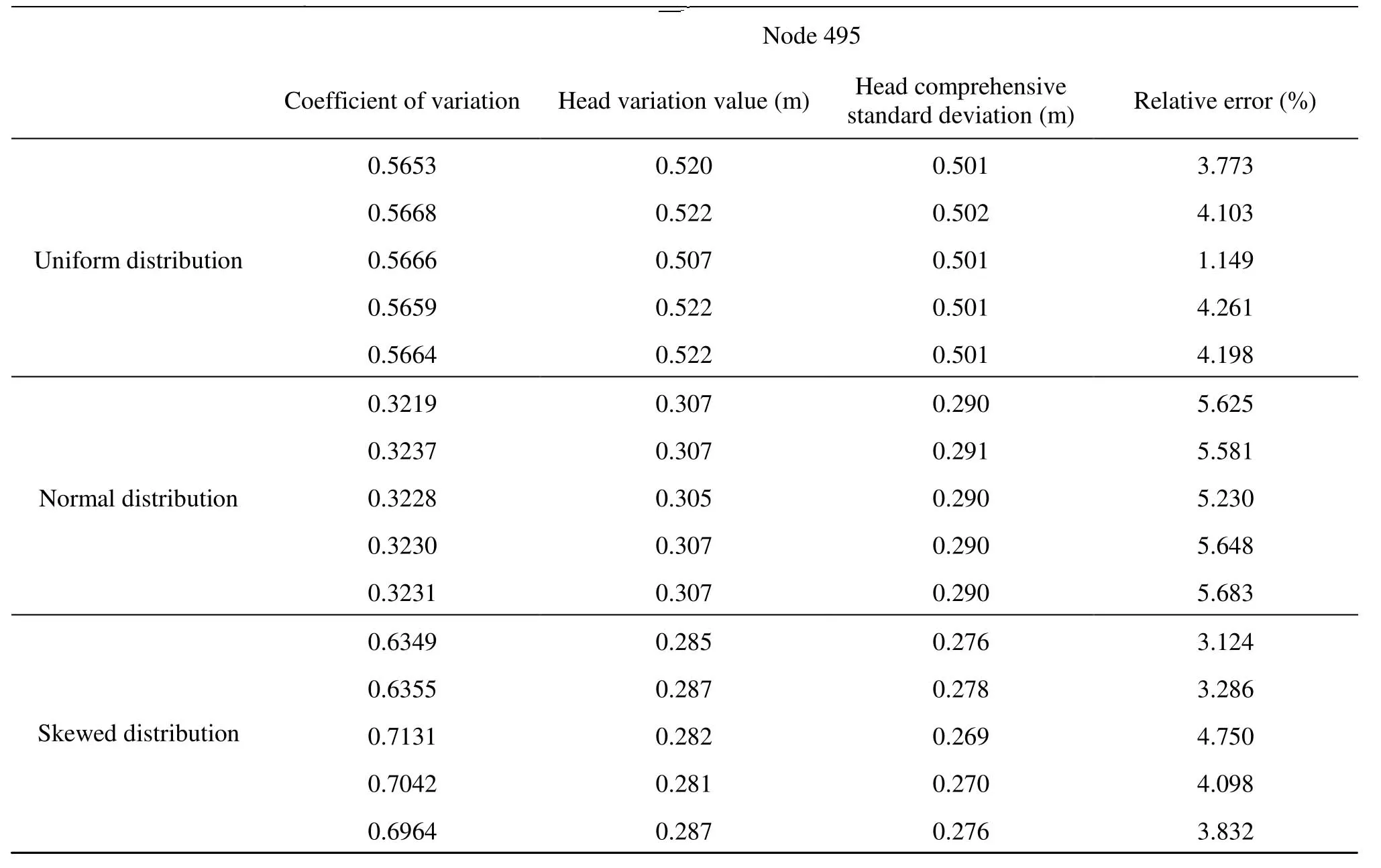
Table 5 Relative error analysis of head variation and head comprehensive standard deviation at node 495

The relationship of stochastic seepage flow fieldsimulated by the Monte Carlo method and SFCM is discussed in the following. The node 489 located on the upstream side of the curtain and the node 495 located on the downstream side of the curtain are selected for comparison (see Fig.7)

Table 6 Comparison of computing efficiency

The relationships of head and head mode in different coefficients of variation and different probability distributions are analyzed, and the results are presented in Table 2 and Table 3.

The results for nodes 489 and 495 indicate that the relative errors of the head and the head mode are within 1% while the coefficient of variation is smaller than 0.71. Therefore, it can be concluded that the deterministic seepage flow field can be perfectly simulated with the real part of head calculated by the SFCM.

The relationships of the head variation and the head comprehensive standard deviation for different coefficients of variation and different probability distributions are shown in Table 4 and Table 5.

The results for nodes 489 and 495 indicate that the relative errors of the head variation and the head comprehensive standard deviation are within 11% while the relative error of the coefficient of variation is smaller than 0.71. Based on the above discussion, the results of skewed distribution appear more ideal. The relative errors of head variation and comprehensive standard deviation are within 5%, and it can better simulate the field or practical conditions and thus reduce the uncertainty of the seepage flow field.

5.3 Analysis of computational efficiency

The computational efficiency of stochastic seepage flow field simulation by the Monte Carlo method and the SCFM method with hydraulic conductivity in normal distribution are selected for comparison as shown in Table 6.

The model presented in this article is simple with fewer computing nodes and elements. But it still can be seen that the computing time and iterations by the SFCM are much less than the Monte Carlo method. The reasons are: (1) the Monte Carlo method needs a large number of random numbers to be generated using the sampling data, (2) and the calculation results should be analyzed to get the statistical parameters. On the other hand, the SFCM only needs inputs of hydraulic conductivity expressed in the complex variable form, and then the head and head variation can be obtained. As a result, the computing time is greatly reduced and the computational efficiency is improved. This advantage will be significant when solving a complex/large model. Therefore, the SFCM is a highly efficient method of stochastic seepage flow field simulation.

6. Conclusions

A new stochastic seepage flow field simulation method named the SFCM is reported in this article. The hydraulic conductivity is considered as random variable and expressed in the complex variable form. The hydraulic conductivities in the Monte Carlo method for stochastic seepage flow field simulation obey respectively the uniform distribution, normal distribution and skewed distribution. The probability density function of skewed distribution and the detailed steps to generate and extract random numbers are presented. The independence and the uniformity of random numbers are guaranteed using this sampling method. Finally, comparing the Monte Carlo method with the SCFM in simulating the stochastic seepage flow field of a section of earth-rock dam demonstrates the feasibility and advantage of solving problems with large variability from a numerical perspective. The main conclusions are as follows:

(1) The head (i.e., the real part of head) obtained using the SFCM is equal to the head mode calculated by the Monte Carlo method with a relative error of about 1%. The relationship between the head variation (i.e., the imaginary part of head) and the comprehensive standard deviation is linear with the regression relationship slopes varying from about 0.9 to 1.0. The skewed distribution shown in this article has the best fitting effect with a relative error of about 5%. Thus, it can be concluded that the stochastic seepage flow field can be simulated well by the SFCM. The results of the stochastic seepage flow field obtained using the Monte Carlo method is necessary to take skewed analysis.

(2) The real part of the analysis results are obtained by the SFCM is the deterministic seepage flow field, and the imaginary part is the range of variation of the deterministic seepage flow field. The range of coefficient of variation of hydraulic conductivity is 0.32 to 0.71, which is larger than previously documented ones with stochastic seepage flow field simulation. The results show that the SFCM is a relatively simple method with high efficiency when the coefficient of variation is smaller than 0.71.

[1] DOGAN A., MOTZ L. H. Saturated-unsaturated 3D groundwater model I: Development[J]. Journal of Hydrologic Engineering, ASCE, 2005, 10(6): 492-504.

[2] FIORI A., DAGAN G. Transport of a passive scalar in a stratified porous medium[J]. Transport in Porous Media, 2002, 47(1): 81-98.

[3] ZHANG D., WAALLSTROM T. C. and WINTER C. L. Stochastic analysis of steady state unsaturated flow in heterogeneous media: Comparison of the Brooks-Corey and Gardner-Russo models[J]. Water Resources Research, 1998, 34(6): 1437-1449.

[4] ZHANG D. Nonstationary stochastic analysis of transient unsaturated flow in randomly heterogeneous media[J]. Water Resources Research, 1999, 35(4): 1127-1141.

[5] ZHANG D., LU Z. An efficient, higher-order perturbation approach for flow in randomly heterogeneous porous media via Karhunen-Loeve decomposition[J]. Journal of Computational Physics, 2004, 194(2): 773-794.

[6] AMIR O., NEUMAN S. P. Gaussian closure of one-dimensional unsaturated flow in randomly heterogeneous soils[J]. Transport in Porous Media, 2001, 44(2): 355-383.

[7] AMIR O., NEUMAN S. P. Gaussian closure of transient unsaturated flow in random soils[J]. Transport in Porous Media, 2004, 54(1): 55-77.

[8] YANG J., ZHANG D. and LU Z. Stochastic analysis of saturated-unsaturated flow in heterogeneous media by combining Karhunen-Loeve expansion and perturbation method[J]. Journal of Hydrology, 2004, 294(1-3): 18-38.

[9] LI Y., LEBOEUF E. J. and BASU P. K. et al. Stochastic modeling of the permeability of randomly generated porous media[J]. Advances in Water Resources, 2005, 28(8): 835-844.

[10] WANG Ya-jun, ZHANG Wo-hua and CHEN He-long. Three-dimensional random seepage field analysis for main embankment of Yangtze River[J]. Chinese Journal of Rock Mechanics and Engineering, 2007, 26(9): 1824-1831(in Chinese).

[11] SHI Ying. Objection of mode definition[J]. Audit And Economy Research, 1996, (3): 52-54(in Chinese).

[12] SHENG Jin-chang, SU Bao-yu and WEI Bao-yi. Stochastic seepage analysis of jointed rock masses by usage of Taylor series stochastic finite element method[J]. Chinese Journal of Geotechnical Engineering, 2001, 23(4): 485-488(in Chinese).

[13] LI Jin-hui, WANG Yuan and HU Qiang. The random variational principle and finite element method in 3D steady seepage[J]. Engineering Mechanics, 2006, 23(6): 21-24(in Chinese).

[14] WANG Yuan, WANG Fei and NI Xiao-dong. Prediction of water inflow in tunnel based on stochastic finite element of unsteady seepage[J]. Chinese Journal of Rock Mechanics and Engineering, 2009, 28(10): 1986-1994(in Chinese).

[15] MAO Chang-xi. Seepage computation analysis and control[M]. Beijing, China: China Water Power Press, 2003(in Chinese).

[16] HU Yun-jin, SU Bao-yu and ZHAN Mei-li et al. Relationship between RRC permeability coefficients of indoor experiment and from water pressure test in situ[J]. Journal of Hydraulic Engineering, 2001, (6): 41-44(in Chinese).

10.1016/S1001-6058(13)60356-X

* Project supported by the National Natural Science Foundation of China (Grant Nos. 51079039, 51009053).

Biography: SONG Hui-bin (1985-), Female, Ph. D. Candidate

ZHAN Mei-li,

E-mail: zhanmeili@sina.com