The Velocity Measurement of Two-phase Flow Based on Particle Swarm Optimization Algorithm and Nonlinear Blind Source Separation*

WU Xinjie (吴新杰)**, CUI Chunyang (崔春阳) HU Sheng (胡晟) LI Zhihong (李志宏) and WU Chengdong (吴成东) College of Physics, Liaoning University, Shenyang 006, China Key Laboratory of Condition Monitoring and Control for Power Plant Equipment, Ministry of Education, North China Electric Power University, Beijing 006, China School of Information Science and Engineering, Northeastern University, Shenyang 0006, China

The Velocity Measurement of Two-phase Flow Based on Particle Swarm Optimization Algorithm and Nonlinear Blind Source Separation*

WU Xinjie (吴新杰)1,**, CUI Chunyang (崔春阳)1, HU Sheng (胡晟)1, LI Zhihong (李志宏)2and WU Chengdong (吴成东)31College of Physics, Liaoning University, Shenyang 110036, China2Key Laboratory of Condition Monitoring and Control for Power Plant Equipment, Ministry of Education, North China Electric Power University, Beijing 102206, China3School of Information Science and Engineering, Northeastern University, Shenyang 110006, China

In order to overcome the disturbance of noise, this paper presented a method to measure two-phase flow velocity using particle swarm optimization algorithm, nonlinear blind source separation and cross correlation method. Because of the nonlinear relationship between the output signals of capacitance sensors and fluid in pipeline, nonlinear blind source separation is applied. In nonlinear blind source separation, the odd polynomials of higher order are used to fit the nonlinear transformation function, and the mutual information of separation signals is used as the evaluation function. Then the parameters of polynomial and linear separation matrix can be estimated by mutual information of separation signals and particle swarm optimization algorithm, thus the source signals can be separated from the mixed signals. The two-phase flow signals with noise which are obtained from upstream and downstream sensors are respectively processed by nonlinear blind source separation method so that the noise can be effectively removed. Therefore, based on these noise-suppressed signals, the distinct curves of cross correlation function and the transit times are obtained, and then the velocities of two-phase flow can be accurately calculated.Finally, the simulation experimental results are given. The results have proved that this method can meet the measurement requirements of two-phase flow velocity.

particle swarm optimization, nonlinear blind source separation, velocity, cross correlation method

1 INTRODUCTION

With the rapid development of science and technology, the two-phase flow system is becoming more and more important for human life and national economy. In metallurgy, chemical engineering, building materials and electricity generation industry, the bulk raw materials are ground into powder. Pneumatic transportation systems can greatly improve the transportation efficiency, reduce pollution, cut down cost and improve the quality of products. Flow measurement is important in industry. In addition, the velocity at which solids are transported in a pneumatic pipeline is significant for the user of the pipeline [1-4]. Excessively high particle velocity will cause high-energy consumption, severe pipeline wear and particle degradation. In contrast, insufficient velocity will cause particle stratification in the pipeline or even pipeline blockage which can result in an explosion.

Cross correlation method has provided a powerful tool in solids velocity measurement, for its wide measurement range and good adaptability [5]. Sensors used in cross correlation method make flow free from an obstruction, so non-contact measurement can be realized. Because the signals obtained by sensors usually contain noise, which will bring great difficulties in searching for the peak of the cross correlation function curves. Although the filtering method based on the hardware can eliminate ordinary noise, the bandwidth of signal is needed to be determined before the circuit design. It is very inconvenient to change the circuit after it has been designed. Both digital filtering method and wavelet transform need to know the bandwidth of signal as prior information to determine the related parameters. Because the output signals of the capacitance sensor are often polluted by noise, and the relationship among the output signals of capacitance sensors, fluid in pipeline and noise is nonlinear,the nonlinear blind source separation, which can overcome shortcomings of the traditional filters, is used to eliminate noise. To overcome the disturbance of noise, this paper presents a method to measure two-phase flow velocity using particle swarm optimization, nonlinear blind source separation and cross correlation method.

2 BASIC PRINCIPLE

2.1 The principles of particle swarm optimization algorithm

Particle Swarm Optimization (PSO) [6] was firstly proposed by Kennedy and Eberhart in 1995. It is a kind of evolution calculation method based on swarm intelligence, and the basic concepts of PSO roots in the research on colony movement of bird.Particles are introduced to simulate birds in group.They fly in the problem space with a certain speed,and every particle has memory and represents one of candidate solution in the solution space. The current velocity and position of particle can be incessantly renewed and the global optimal solution can be obtained at last. PSO algorithm needs less prior parameters and can be easily controlled. The rate of convergence is quick because it is of good parallelism. During the past decade, PSO algorithm has achieved great success in many industrial fields.

Suppose the following scenario: a group of birds are randomly searching food in an area. There is only one piece of food in the area. None of them know where the food is. But they know how far the food is from their current position in each iteration. So the best strategy to find the food is to search for the area around the bird which is the nearest one to the food.PSO algorithm learned from the scenario and used it to solve the optimization target [7]. In PSO algorithm,each potential solution is a ‘bird’ in the search space,and we call it as ‘particle’. All particles have fitness values which are evaluated by the function to be optimized, and have velocities which direct the flight of the particles and control the distances of the particles.The particles fly through the problem space by following the current optimum particles. PSO algorithm is initialized with a group of random particles (random solutions) and then searches for optimal value by iterations. In each iteration, each particle is updated by the following two ‘best’ values. One is the best solution which is gotten by itself so far. Another is the best value which is obtained by any particle in the population so far.

The mathematical representation of PSO algorithm is given as follows: Suppose there is D-dimensional search space, a community is composed of m particles,the ith particle represents a D-dimensional vector, i = 1 ,2,···,m , namely, Xiis the position of the ith particle in the search space. In other words, the position of each particle is a potential solution.We can calculate the fitness value by Xiand target function. The position Xiis evaluated by the fitness value.The flight speed of the ith particle is D-dimensional vector as well, which is expressed asthe current best position of the ith particle and the best position of the entire swarm respectively.

The particle updates its velocity and positions with the following equations:

which were firstly proposed by Kennedy and Eberhart[6], in which i = 1 ,2,· · ·,m , d = 1 ,2,···,D , the acceleration factors c1and c2(or learning factors) are nonnegative constants, r1and r2are random number between [0,1], t is the iteration time. vid∈[− vmax, vmax],vmaxalso is a constant which is specified by the user,if the value ofmaxv is too large, the particle will possibly fly over the best solution. If the value ofmaxv is too small, the particle will possibly sink into local optimal value.

Shi et al. [8] developed Eq. (1) and then gave their opinion as follows:

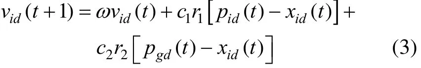
where ω is a nonnegative value called inertia factor.We can balance the convergence rate and the ability of local search by adjusting the value of ω, because the ability of local search can be improved with small ω and the fast convergence rate can be obtained from large ω. ω can be obtained by linear descend functions or other nonlinear functions [8, 9]. Within a certain interval, it can make the algorithm be of much faster convergence rate in the early stage and stronger ability of local search in the later stage.

2.2 The principles of blind source separation algorithm

Since the blind source separation [10] has been raised in 1980s, it has become one of the most active methods in the research area of signal processing. The blind source separation means that when the characteristics of source signals and transmission channels are unknown, every component is estimated by some priori knowledge of observed signals and source signals. One of its key problems is the algorithm of separation matrix, which belongs to unsupervised learning. The basic idea of blind source separation is that the statistical independent features to be extracted are used as the input. Actually, most of the observed signals may be obtained by nonlinear mixed superposition. This problem is much more complicated than the linear problem, so the blind source separation methods of linear mixtures can’t be applied to nonlinear mixed signals. At present, the research methods of blind source separation of nonlinear mixtures can be roughly divided into two categories. One is selforganizing feature mapping. This method can extract the nonlinear components by self-organizing feature mapping [11] without considering the form of the nonlinear mixtures. If the number of the source signals is large, the network complexity will have an exponential growth with the increasing number of source signals, and there will be interpolation error in separating the continuous source signals. The other one is that a nonlinear mixed model is based on the blind source separation of linear mixtures [12, 13]. This method usually gets the solution by Newton’s iteration method and gradient algorithm. But when they are used in the problem of nonlinear blind source separation, the global optimal solution can’t be easily obtained. So the particle swarm optimization algorithm is used in nonlinear blind source separation in this paper.

Supposing s (t) = [s(t),s(t) , ···,s(t )]Trepresents

1 2n n source signals, and x (t) = [x(t),x (t) , ···,x (t )]T

1 2m represents m observed signals. Each of the observed signals is a mixture of the source signals, and the specific mixing method is unknown. Eq. (4) represents mixing process:

where A is mixing matrix, and n(t) is noise.

If W represents the separation matrix, and y(t)represents the output signals after the separation,while noise is ignored, y(t) Wx(t). The purpose of blind source separation is that the source signals s(t)can be separated from the observed signals x(t) under conditions that source signals and mixing matrix are unknown. The separation methods to be adopted can make separation signals close to the source signals as far as possible. In other words, the process of blind source separation is to look for separation matrix W.When the signal with noise is separated, we can deal with the noise as a signal. However, the model of linear transformation may fail in some situations, the model of nonlinear transformation is more suitable for actual situations. And the relationship between the observed signals and source signals can be defined as [14]

where F = [ f, f , ···, f ]Tis a reversible nonlinear

1 2n transformation functions matrix. If F = [ f, f , ···, f ]T

1 2n is linear one, then Eq. (5) is equivalent to Eq. (4).

The nonlinear model is shown in Fig. 1. The mixing system can be divided into two parts. The source signals s(t) are mixed by the linear mixing matrix A, then the output signal of each channel is transformed by an independent nonlinear transform functions fi. While the de-mixing system includes the independent inverse transform functions giof each channel and the separation matrix W, then the output signals yi(t) can be defined as

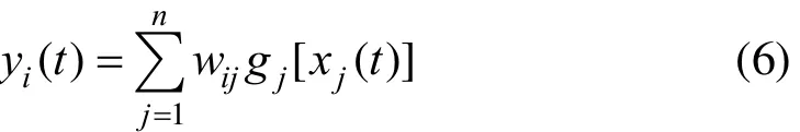
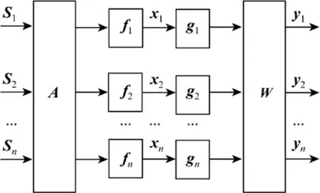
Figure 1 The nonlinear mixing and de-mixing model

Because there is no prior knowledge of the mixing system and the de-mixing system, the inverse transform function is uncertain. But most of them are symmetrical about the origin, so they can be fitted by odd polynomials of higher order.

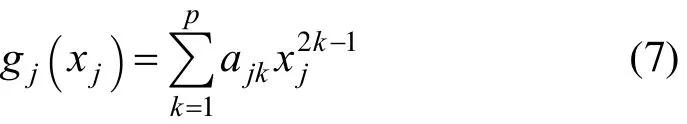
gi[ xi(t)] in Eq. (6) can be replaced by Eq. (7) to get:

where a = [ a ,a ,···,a ]Tis the parameters of

j j1 j2 jp nonlinear inverse transform function of the jth channel.

3 NONLINEAR BLIND SOURCE SEPARATION BASED ON PARTICLE SWARM OPTIMIZATION ALGORITHM

There are many different forms of the evaluation function in nonlinear blind source separation algorithms, such as the higher-order cumulants, mutual information and so on. We select mutual information[15] as the evaluation function:

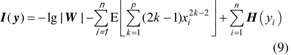
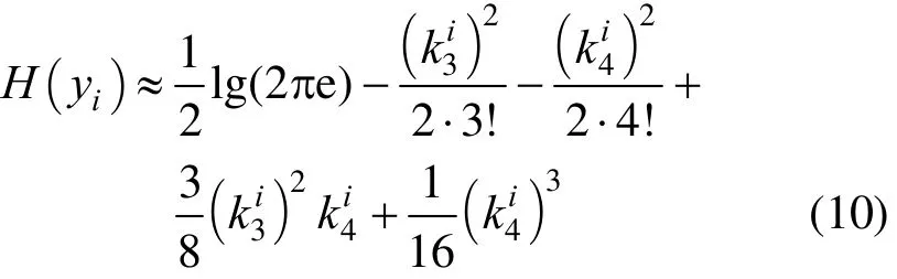
When the elements in y are statistically independent with each other, the mutual information I(y) 0. Using Gram-Charlie expansions, then H(yi) is changed to

Before computing the mutual information of the signals, we should carry on the centralization and pre-whitenization of the signals. The goal of centralization of the signals makes the signals have zero mean values. This can be accomplished by subtracting their mean values in original signals. The purpose of pre-whitenization of the signals is to seek for the whitenization matrix D, which makes transformation output =y xD be uncorrelated. As a result, the variance of y is one. When the value of I(y) gets the minimum, the signals are mutually independent. Under the constraint of E(yyT)=I, then Eq. (9) can get the extremum.

The main steps of nonlinear blind source separation based on the PSO algorithm are as follows:

(1) Get the observed signals.

(2) Carry on the centralization and the prewhitenization of the observed signals.

(3) Initialize the particle group, the parameters of de-mixing function and separation matrix. Create random initial particles, Gj=and separation matrix W.

(4) Carry on the centralization and the prewhitenization after each separation. Calculate the fitness value of each particle according to Eq. (9).

(5) Update the velocity and position of each particle according to Eqs. (3) and (2).

(6) Enter the circulation, return to Step 4, until a termination criterion is met. Output the optimal solution in the end.

4 EXPERIMENTAL RESULTS AND ANALYSIS

The relationship between the output signals of capacitance sensors and fluid flow in pipeline is nonlinear, and this relationship can be approximately modelled as tanh(ax). This conclusion can be obtained from Fig. 2. Fig. 2 (a) shows relation between the output signal of capacitance sensor and the permittivity of the fluid. The data in Fig. 2 (a) are obtained using the simulation software COMSOL. The x-axis represents the permittivity of the fluid, and the y-axis represents the output signal of capacitance sensor. Fig.2 (b) gives the output curves of the function tanh(0.5x)with change of x. We can see the shapes of two curves are similar. So tanh(ax) is used as the model of nonlinear transformation function.

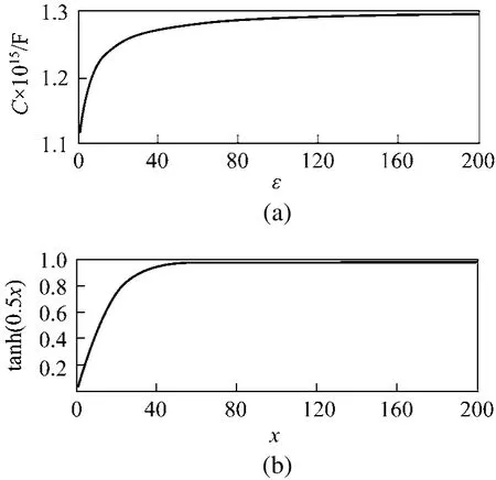
Figure 2 The contrast of the output signal of capacitance sensor and the function tanh(0.5x)

In order to verify the effectiveness of the method proposed in this paper, the data of simulation experiment are provided. The original signals are obtained from upstream and downstream capacitance sensors of coal powder injection system in No. 3 blast furnace of Baoshan Iron ＆ Steel Co., Ltd. The outer and inner diameters of pipeline are 108 mm and 96 mm respectively. The length and width of the capacitance electrode are respectively 210 mm and 128 mm. The distance between upstream and downstream capacitance electrodes is 240 mm. Two electrodes of upstream and downstream capacitance sensors are symmetrically fixed on pipeline respectively. Firstly, the upstream sensor signals S1and white noise signals S2which are generated by ‘rand(n,n)’ function in Matlab are mixed by a linear mixing matrix:

And nonlinear transform functions F1=tanh(0.2 x1)and F2=tanh(0.5 x2), thus we get two group mixed signals of upstream sensor; and we can also do the same thing on the downstream sensor. Secondly, the signals of upstream and downstream sensors are separated from mixed signals by the method based on particle swarm algorithm and nonlinear blind source separation respectively. The cross correlation curves can be obtained by cross correlation calculation of two separation signals of upstream and downstream sensors. The transit time of flow from upstream sensor to downstream sensor can be calculated by the correlation curve. The velocities of two phase flow are obtained according to the transit time. Table 1 is a velocity measurement results comparison. The second column in Table 1 is velocities obtained by original signals.The third column in Table 1 is velocities obtained by separation signals which are obtained by the method proposed in this paper. There might be some error in three groups of experiment results in Table 1, which can be possibly produced by the error of nonlinear blind source separation method.

Table 1 Velocity comparison table

Figure 3 The mixed signals, separation signals and cross correlation curves

Figures 3 (a) and 3(b) respectively expresses one of output signals of upstream and downstream sensors after noises are added. The result in Fig. 3 corresponds to the result of the 4th set of data in Table 1. The separation signals of upstream and downstream sensors which are obtained by the method proposed in this paper are shown in Figs. 3 (c) and 3 (d) respectively. And Figs. 3 (e) and 3 (f) are cross correlation curves before and after the proposed method is used.

Before noises are added to the signals, the transit time is 26.0 ms, and after noises are added to the signals, the transit time which obtained by the proposed method [see Fig. 3 (f)] is still 26.0 ms. In Fig. 3 (e),the extreme cannot be identified from the cross correlation curve when the mixed signals are processed by digital filtering method, so transit time can’t be obtained. And other simulation results and the case mentioned above are the same.

5 CONCLUSIONS

Under the actual condition, measurement signals are usually composed with signals and noise, so the output signals of sensors are usually considered as mixed signals. This paper presented a method to extract useful signals from noises using nonlinear blind source separation. The simulation experimental results have proved the validity of this method. The disturbance of noises significantly decreases after output signals of capacitance sensors are processed by the method proposed in this paper, so the transit time can be more exactly obtained, and the calculation results of two-phase flow velocities are more accuracy. The signal processing system of this method is simpler and cheaper. Its noise filtering effect is better than the traditional digital filter. Therefore, the proposed method presents a new way and an effective means for two phase flow velocity measurement. This method has a wide development prospect and higher industrial application value. But this velocity measurement method is only accomplished by simulation. At present, since it has not yet been used in actual measurement, it still needs further study and improvement.

1 Yan, Y., “Mass flow measurement of bulk solids in pneumatic pipelines”, Meas. Sci. Technol., 7 (12), 1687-1706 (1996).

2 Thorn, R., Beck, M.S., Green, R.G., “Non-intrusive methods of velocity measurement in pneumatic conveying”, J. Phys. E Sci. Instrum., 15 (11), 1131-1139 (1982).

3 Green, R.G., Rahmat, M.F., Dutton, K., Evansy, K., Goudey, A.,Henry, M., “Velocity and mass flow rate profiles of dry powders in a gravity drop conveyor using an electrodynamic tomography system”,Meas. Sci. Technol., 8 (4), 429-436 (1997).

4 Wang, X., Guo, L.J., Zhang, X.M., Guo, F.D., “Experimental study of liquid slug velocity in horizontal pipeline”, Journal of Engineering Thermophysics, 27 (1), 71-74 (2006). (in Chinese)

5 Xu, L.A., Yang, H.L., Zhang, T., Li, W., “Clamped-on ultrasound cross-correlation flowmeter and its application to liquid/solid two-phases flow measurement”, Chinese Journal of Scientific Instrument, 14 (3), 257-262 (1993). (in Chinese)

6 Kennedy, J., Eberhart, R.C., “Particle swarm optimization”, In: Proceedings of IEEE international conference on neural networks, Perth,Australia, 4, 1942-1948 (1995).

7 Li, A.G., Tan, Z., Bao, F.M., He, S.P., “Particle swarm optimization”,Computer Engineering and Applications, 38 (21), 1-3 (2002). (in Chinese)

8 Shi, X.H., Liang, Y.C., Lee, H.P., Lu, C., Wang, L.M., “An improved GA and a novel PSO-GA-based hybrid algorithm”, Infor. Process.Lett., 93, 255-261 (2005).

9 Liu, B., Wang, L., Jin, Y.H., Tang, F., Huang, D.X., “Improved particle swarm optimization combined with chaos”, Chaos, Solitons Fractals, 25(5), 1261-1271 (2005).

10 Jutten, C., Herault, J., “Blind separation of sources”, Signal Process.,24 (1), 1-10 (1991).

11 Karhunen, J., “Neural approaches to independent component analysis and source separation”, In: Proc. ESANN, Bruges, Belgium,49-266 (1996).

12 Haritopoulos, M., Yin, H., Allison, N., “Image denoising using self-organizing map-based nonlinear independent component analysis”,Neural Networks, 15 (8-9), 1085-1098 (2002).

13 Burel, G., “Blind separation of sources: A nonlinear neural algorithm”, Neural Networks, 5 (6), 937-947 (1992).

14 Wei, Y., Liu, Z.X., Li, N., Sun, D.B., “Nonlinear blind source separation using improved particle swarm optimization”, Aerospace Electron. Infor. Eng. Control, 28 (1), 138-142 (2006).

15 Yang, H.H., Amari, S., Cichocki, A., “Information theoretic approach to blind separation non-linear mixture”, Signal Process., 64(2), 291-300 (1998).

2011-12-14, accepted 2012-01-10.

* Supported by the National Natural Science Foundation of China (50736002, 61072005); the Youth Backbone Teacher Project of University, Ministry of Education, China; the Scientific Research Foundation of the Department of Science and Technology of Liaoning Province (20102082); and the Changjiang Scholars and Innovative Team Development Plan (IRT0952).

** To whom correspondence should be addressed. E-mail: wuxinjie@lnu.edu.cn