Conserved vectors and symmetry solutions of the Landau–Ginzburg–Higgs equation of theoretical physics

Chaudry Masood Khaliqueand Mduduzi Yolane Thabo Lephoko

Material Science,Innovation and Modelling Research Focus Area,Department of Mathematical Sciences,North-West University,Mafikeng Campus,Private Bag X 2046,Mmabatho 2735,South Africa

Abstract This paper is devoted to the investigation of the Landau–Ginzburg–Higgs equation (LGHe),which serves as a mathematical model to understand phenomena such as superconductivity and cyclotron waves.The LGHe finds applications in various scientific fields,including fluid dynamics,plasma physics,biological systems,and electricity-electronics.The study adopts Lie symmetry analysis as the primary framework for exploration.This analysis involves the identification of Lie point symmetries that are admitted by the differential equation.By leveraging these Lie point symmetries,symmetry reductions are performed,leading to the discovery of group invariant solutions.To obtain explicit solutions,several mathematical methods are applied,including Kudryashov’s method,the extended Jacobi elliptic function expansion method,the power series method,and the simplest equation method.These methods yield solutions characterized by exponential,hyperbolic,and elliptic functions.The obtained solutions are visually represented through 3D,2D,and density plots,which effectively illustrate the nature of the solutions.These plots depict various patterns,such as kink-shaped,singular kink-shaped,bell-shaped,and periodic solutions.Finally,the paper employs the multiplier method and the conservation theorem introduced by Ibragimov to derive conserved vectors.These conserved vectors play a crucial role in the study of physical quantities,such as the conservation of energy and momentum,and contribute to the understanding of the underlying physics of the system.

Keywords: Landau–Ginzburg–Higgs equation,Lie symmetry analysis,group invariant solutions,conserved vectors,multiplier method,Ibragimov’s method

1.Introduction

Nonlinear partial differential equations (NLPDEs) are extensively employed in the fields of science and engineering to represent and study a wide range of nonlinear phenomena encountered in practical applications [1–13].These equations play a crucial role in modeling various scenarios,including fluid dynamics problems,wave propagation in complex media,seismic wave analysis,and the characterization of optical fibers.The versatility and applicability of NLPDEs enable researchers and engineers to gain valuable insights into complex physical phenomena and devise effective strategies to address real-world challenges.Numerous mathematical and physical NLPDEs have been investigated in the literature and,currently,mathematicians are tackling even more.For instance,in their research,Zhang and Xiao [8] utilized an undetermined coefficient method to study the (2+1)-dimensional generalized Hirota–Satsuma–Ito equation,which describes the propagation of unidirectional shallow-water waves.They focused on obtaining double-periodic soliton solutions.In a separate study,Raoet al[9]utilized the Cole–Hopf algorithm to analyze the (2+1)-dimensional modified dispersive water-wave system,and obtained its exact solutions.Zhang and Wang [10] employed various methods,including the simplified extended tanh-function method,variational method,and He’s frequency formulation method,to investigate the Fokas system that arises in monomode optical fibers.Through their research,they obtained fifteen sets of soliton solutions.Wang and Liu [11] investigated the new coupled Konno–Oono equation that plays a key role in the magnetic field by applying the Exp-function method to find its analytical solutions.

The pursuit of accurate solutions for NLPDEs holds considerable importance within the realm of applied mathematics.These precise solutions assume a pivotal role in comprehending the qualitative and quantitative attributes of nonlinear phenomena.Despite the existence of diverse classes of intriguing exact solutions,such as soliton and traveling wave solutions,their construction usually requires specialized mathematical techniques due to the nonlinearity inherent in their dynamic nature.However,the presence of nonlinearity in NLPDEs presents a formidable challenge to discovering explicit,specific,or general solutions.Consequently,various robust techniques have been proposed and developed to derive analytical solutions for nonlinear problems.

Stating a few of the well-established techniques,we have the ansatz technique [14],the extended homoclinic-test approach [15],the generalized unified technique [16],the tanh-coth method [17],the exp (-Φ(η))-expansion technique[18],the Bäcklund transformation approach [19],the Cole–Hopf transformation approach [20],the Painlevé expansion approach [21],the mapping and the extended mapping approaches [22],the homotopy perturbation approach [23],the rational expansion method [24],the simplest and the extended simplest equation techniques [25],the F-expansion approach [26],Hirota’s technique [27],Lie symmetry analysis [28,29],the Darboux transformation technique [30],the exponential function technique [31],Kudryashov’s technique[32],the tanh-function method [33],and the bifurcation approach [34].

Conservation laws are of significant importance in the analysis of differential equations.One practical application of this is the assessment of the integrability of a partial differential equation via examination of its conservation laws[29].Furthermore,conservation laws serve as a tool for assessing the precision of numerical solution techniques,help identify special solutions that have important physical properties,and can be used to reduce the number of unknowns in a problem,making it easier to solve [29].Thus,this is the reason mathematicians find it useful to determine the conservation laws for a given differential equation (DE) [35,36].A novel category of nonlinear evolution equations(NLEEs),featuring a nonlinear term of arbitrary order represented in the form

were introduced by Chenet al[37],wherea1,a2,a3,a4,andp≠1 are arbitrary constants.Whenptakes a different constant,a different equation will be constructed.These include the sine-Gordon equation,Duffing equation,and the Klein–Gordon equation.Infact,whenp=3,a4=0 we get the NLEE

One common version of equation (1.2) is the Landau–Ginzburg–Higgs equation (LGHe),given by

withu=u(t,x) representing the electrostatic potential of the ion-cyclotron wave,andaandbare constants [38,39].The LGHe (1.3) is used to understand the concepts of superconductivity and cyclotron waves,which have applications in a variety of fields,including medicine,plasma physics,chemistry,biology,electricity-electronics,and transportation [40].

In [39],the modified exponential function approach was used to obtain the solution of the LGHe(1.3)that were of the hyperbolic,trigonometric,and rational functions forms.Barmanet al[41] employed the extended tanh method and applied the solitary wave hypothesis to obtain explicit traveling wave solutions.They achieved this by assigning various specific values to the parameters involved in the equations.Bekir and Ünsal[38]obtained solitary and periodic wave,and exponential solutions via the first integral method with the computerized symbolic computation system Maple.Islam and Akbar [42] utilized the improved Bernoulli subequation function method to successfully establish stable general,broad-ranging,typical,and fresh soliton solutions to the LGHe.Iftikharet al[43] used the-expansion method to gain traveling wave solutions.Recently,Ahmadet al[44] obtained exact solutions of the LGHe in terms of elliptic Jacobi functions by applying the power index method using function conversion.Asjadet al[45] obtained solitary wave solitons by utilizing the generalized projective Riccati method.

Motivated by the existing literature,this research endeavors to address the LGHe (1.3) using five distinct and efficient techniques: the Lie symmetry technique,Kudryashov’s technique,the extended Jacobi elliptic function technique,the power series method,and the simplest equation approach.The primary objective of this study is to generate a new multitude of exact solutions for the LGHe (1.3).Additionally,the dynamical behaviour of solitary wave profiles for select soliton solutions will be demonstrated through numerical simulations by employing three-dimensional and density plots.Notably,we assert that the evolutionary dynamics and physical interpretation of the acquired exact soliton solutions are highly intriguing and offer valuable insights for further physical propositions.Importantly,the majority of the derived exact soliton solutions are new and,to the best of our knowledge,have not been previously reported in the literature.Finally,for the first time,we establish the conservation laws associated with the underlying model by employing the multiplier method and Ibragimov’s theorem.

2.Lie symmetry analysis of the LGHe

In this section we first use the algorithm for the computation of Lie point symmetries of the LGHe (1.3) and generate its Lie point symmetries.Thereafter,we utilize them to construct exact solutions for equation (1.3).

2.1.Lie point symmetries of the LGHe

Let us consider the one-parameter Lie group of infinitesimal transformations,namely,

where α denotes the parameter of the group,while τ,ξ,and η represent the infinitesimals of the transformations.Utilizing a one-parameter Lie group of infinitesimal transformations that satisfy certain invariant conditions[29],the solution space(t,x,u) of the LGHe (1.3) remains invariant and can be transformed into another space.Imploring the vector field

the symmetry group of the LGHe (1.3) will be found.We recall that equation (2.4) is a symmetry of the LGHe (1.3),provided that the invariance condition

holds.Here,pr(2)W denotes the second prolongation of W[29] defined by

with the ζʼs given by

and the total derivatives defined as

Expanding the determining equation (2.5) and separating it into its constituent derivatives ofu,we obtain an overdetermined system of eight homogeneous linear partial differential equations

Solving the above system for τ,ξ,and η,one obtains

withc1,c2,andc3being arbitrary constants.Thus,we have three symmetries

Theorem 2.1.The LGHe(1.3)admits a three-dimension Liealgebra L3,which is spanned by the vectorfieldsW1,W2,W3,as defined in equation(2.8).The group transformations related to the Lie algebraL3are given as

with α1,…,α3representing real numbers.Thus,we can state the following theorem.

Theorem 2.2.Ifu=N(t,x)is a solution of the LGHe(1.3),then by using the one-parameter symmetry groupsGi(i=1,2,3),we have new solutions given by

2.2.Symmetry reduction of the LGHe

This section focuses on the utilization of the infinitesimal symmetries obtained in the previous section to determine the similarity variables and exact solutions of the LGHe (1.3).This involves solving the characteristic equation,which is akin to solving the invariant surface conditions.

Reduction 1.The symmetry W1=∂tyields two invariantsu=G(q),q=x.Utilization of these invariants transforms the LGHe (1.3) to the reduced nonlinear ordinary differential equation (NLODE)

Reduction 2.The invariantsu=G(q),q=tof the symmetry W2=∂xtransform equation (1.3) to the reduced equation

Reduction 3.Likewise,the symmetry W3=x∂t+t∂xtransforms the LGHe(1.3) to

Reduction 4.Finally,the linear combination W1+cW2=∂t+c∂x,wherecis the wave speed,transforms the LGHe(1.3) to the reduced NLODE

3.Solutions to the reduced equations

We employ various methods to find exact solutions for the reduced NLODEs (2.9),(2.10),(2.11),and (2.12).These methods allow us to explore different approaches to obtaining diverse solutions for the reduced equations.

3.1.Solutions of equation (1.3) using Kudryashovʼs technique

We present a solution to equation (1.3) using Kudryashov’s method [46].This method is widely used to obtain closedform solutions to NLPDEs.The first step involves reducing the NLPDE (1.3) to an NLODE,which we have already accomplished in the previous section.Thus,we will be working with the NLODE(2.9).We assume that the solution to equation (2.9) can be expressed as

wherey(x) satisfies the NLODE

We note that the closed-form solution of equation (3.14) is

For equation (2.9),the balancing procedure leads toN=1.Thus,from equation (3.13),we have

Now,substituting equation (3.16) into equation (2.9) and using equation (3.14),we obtain

Separating the terms according to the powers ofy(x),we obtain four distinct algebraic equations for the coefficientsB0andB1

The solution of the above equations is

Thus,the solutions of the LGHe (1.3) are

which represent the steady state solutions of equation (1.3).

3.2.Solutions of equation (1.3)via application of the extended Jacobi elliptic function technique

In this section,we employ the extended Jacobi elliptic function expansion method,as outlined in [47–49],to solve the NLODE (2.10) and obtain the cnoidal,snoidal,and dnoidal wave solutions of the LGHe(1.3).The methodology involves representing the solution of the NLODE as

whereMis a positive integer,determined via the balancing procedure,and

denote the cosine-amplitude function,the sine-amplitude function,and delta amplitude function,respectively.The aforementioned serve as solutions to the NLODEs

respectively.

3.2.1.Cosine-amplitude periodic wave solutions of equation (1.3).Considering the NLODE (2.10),the solution can be expressed as equation (3.19),where the balancing procedure setsM=1.Thus

whereA-1,A0,andA1are constants that need to be determined.By substituting the given expression forG(t)into equation (2.10) and employing equation (3.22),we obtain an equation that can be separated into different powers ofG(t) and that yields seven distinct algebraic equations

The solutions to these equations,obtained with the assistance of Mathematica,are provided below

Solution set 1.

Solution set 2.

Solution set 3.

Hence,the cnoidal wave solution of the LGHe (1.3)corresponding to solution set 1 is given by

where it should be noted that as ω→1,cn(t∣ω)→sech(t).Therefore,the general solution for solution sets 2 and 3 is a hyperbolic function,which can be expressed as

3.2.2.Sine-amplitude periodic wave solutions of equation (1.3).In a similar manner,we derive snoidal wave solutions for equation (1.3).It is important to note that the balancing procedure results inM=1.We utilize the NLODE presented in equation (3.23),with its solution given by equation (3.20).Following a similar procedure to that described previously,we obtain the following set of seven distinct algebraic equations:

The solutions of these algebraic equations,computed using Mathematica,are

Solution set 1.

Solution set 2.

Solution set 3.

Hence,the solutions of the LGHe (1.3) corresponding to the three solution sets mentioned above are

3.2.3.Dnoidal periodic wave solutions of(1.3).As before,we now proceed to obtain dnoidal wave solutions for the LGHe(1.3).We employ the NLODE stated in (3.24),whose solution is provided by (3.21),and derive the set of seven algebraic equations

The solutions of these algebraic equations,computed using Mathematica,are

Solution set 1.

Solution set 2.

Solution set 3.

Therefore,the solution of the LGHe (1.3) that corresponds with the solution sets is

3.3.Solution of equation (1.3) using the power series method

The power series solution technique [50–52] for DEs is now employed to construct solutions of the LGHe (1.3).Power series methods have proven to be effective in addressing challenging DEs,encompassing a wide range,from difficult semi-linear to complex nonlinear differential equations.Hence,in this section,we aim to obtain the exact analytical solutions for the NLODE (2.11) using the power series technique.Consequently,we employ the formal series solution

where ρi(i=0,1,2,...) are constants to be determined.The derivatives of equation (3.26) to be used are given as

By substituting the expressions forG,G′,andG″ from equations (3.26) and (3.27) into equation (2.11),we obtain

By further simplifying equation (3.28),we obtain

Comparing the coefficients ofzin equation (3.29),we obtain

Generally,forn≥2,the recursion relation in view of equation (3.29) is

Utilizing equations (3.30),(3.31),and(3.32),it is possible to determine all the coefficients ρn(n≥2) of the power series,equation (3.26).For arbitrarily selected constants ρ0,ρ1,ρ2,and ρ3,the remaining terms can also be determined in a unique manner through successive application of equations (3.30),(3.31),and (3.32).

Convergence of the power series solution

Now,we shall provide proof of the convergence of the power series solution,equation(3.26).Hence,we introduce a new series

withqi=∣ρi∣(i=0,1)and

It suffices to prove the following propositions:

Proposition 1.The series,equation(3.33),is a majorant series of equation(3.26).

Proof.To establish that the new series,equation(3.33),serves as a majorant series for equation (3.26),it suffices to demonstrate that ∣ρn∣≤qn,forn=0,1,2,….Without loss of generality,from equation (3.32),we establish the following:

where

Thus,by comparing equation (3.35) with equation (3.32),it becomes evident that

This implies that equation (3.33) serves as a majorant series for equation (3.26).

Proposition 2.The series,equation(3.33),has positiveradius of convergence in the interval(0,q0).

Proof.To proveλ=Q(z)has positive radius of convergence,we writeQ(z) in the form

Now,we turn our attention to the implicit functional equation

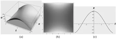
Figure 1. (a) A 3D graph of the bell-shaped solution (3.38) for a=1,b=2,ρ0=2,ρ1=1,and -5≤t,x≤5.(b) A 2D density plot of solution (3.38).(c) A 2D graph of solution (3.38) for x=3 and -5≤t≤5.

It is sufficient to show that P(z,λ) is analytic in the neighborhood of (0,q0).From equation (3.36),it is evident that

By applying the implicit function theorem [53,54],we can establish thatλ=Q(z)is an analytic function in the vicinity of(0,q0).Additionally,by combining propositions 1 and 2,we can infer that equation(3.33)acts as a majorant series for equation (3.26) and possesses a positive radius of convergence.As a result,the power series,equation (3.26),converges in a neighborhood of(0,q0).Thus,the power series solution of equation (2.11) can be written as

Hence,the exact power series solution of equation (1.3) is given by

whereρi,fori=0,1,represent arbitrary constants.The remaining coefficientsρn,forn≥2,can be determined iteratively using equations(3.30),(3.31)and(3.32).However,in practical applications,it is often more convenient to work with an approximate form of the solution

The wave character of the solution in equation (3.38) is shown in figure 1.

3.4.Solutions of equation (1.3) using the simplest equation approach

We employ the simplest equation approach,as described in[55],to solve the second-order NLODE (2.12).The simplest equations used in this method are the Bernoulli and Riccati equations,given respectively by:

wherel,m,andnare constants.We seek solutions of the NLODE (2.12) in the form

whereH(ξ)satisfies either the Bernoulli equation(3.39)or the Riccati equation (3.40),Mis a positive integer,determined via the balancing procedure,andA0,…,AMare parameters to be determined.The solutions of the Bernoulli equation(3.39)that we utilize here are

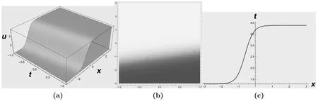
Figure 2. (a)A 3D graph of the kink-shaped solution(3.47)for l=4,b=2,c=-0.4,m=1,c0=1,c1=1,and-3≤t,x≤3.(b)A 2D density plot of solution (3.47).(c) A 2D graph of solution (3.47) for t=1 and -3≤x≤3.

wherec0,c1,andc2are constants.For the Riccati equation (3.40),the solutions we consider are

3.4.1.Solutions of equation (1.3) using the Bernoulli equation.In this case,the balancing procedure yieldsM=1,and the solutions of equation (2.12) take the form

By substituting equation (3.46) into equation (2.12) and utilizing the Bernoulli equation (3.39),we can equate the coefficients ofHito zero.This leads to a system of four algebraic equations in terms ofA0andA1:

Using Mathematica,we can solve the above system of equations and obtain the following solutions:

Solution set 1.

Solution set 2.

Therefore,the solutions of the LGHe (1.3) corresponding to solution sets 1 and 2 are

where ξ=x-ctandc0is an arbitrary constant.The wave profile of the hyperbolic solutions,equations (3.47) and(3.48),can be seen in figures 2 and 3.

3.4.2.Solutions of equation(1.3)using the Riccati equation.In this case,the balancing procedure givesM=1 and,therefore,equation (3.41) becomes

Inserting the above expression forG(ξ) into equation (2.12)and making use of the Riccati equation (3.40) yields the following system of four algebraic equations:

The solution of the aforementioned system,using Mathematica,is

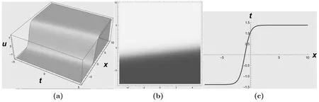
Figure 3. (a)A 3D graph of the kink-shaped solution(3.48)for l=2,b=1,c=0.2,m=1,c0=1,c2=1,and-5≤t≤5,-8≤x≤10.(b) A 2D density plot of solution (3.48).(c) A 2D graph of solution (3.48) for t=0 and -8≤x≤10.

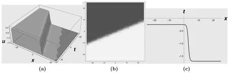
Figure 4. (a)A 3D graph of the kink-shaped solution(3.50)for l=4,b=2,c=0.4,m=3,n=1,c0=1,c1=1,and-25≤t,x≤25.(b)A 2D density plot of solution (3.50).(c) A 2D graph of solution (3.50) for t=10 and -25≤t≤25.

Consequently,the solutions of the LGHe(1.3)corresponding to the above values are

where ξ=x-ctandc0is an arbitrary constant.The dynamical wave profiles for the solutions,equations (3.50)and (3.51),are shown in figures 4 and 5,respectively.

3.4.3.Solutions of equation (1.3) using the extended Jacobi elliptic function technique.In a similar manner to that discussed in the previous section,our focus now moves towards the acquisition of exact solutions using the extended Jacobi elliptic function expansion method on the NLODE(2.12).

Cnoidal wave solutions of (1.3)

Considering the NLODE(2.12),recall that the balancing procedure leads toM=1.Thus

whereA-1,A0,andA1are constants that need to be determined.By substituting the above expression forG(ξ)into equation (2.12) and employing equation (3.22),we obtain an equation that can be separated on different powers ofG(ξ) and that yields seven distinct algebraic equations

The solutions to the above equations,obtained with the assistance of Mathematica,are

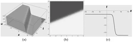
Figure 5. (a)A 3D graph of the kink-shaped solution(3.51)for l=4,b=2,c=0.4,m=3,n=1,c0=1,c1=1,and-15≤t,x≤15.(b)A 2D density plot of solution (3.51).(c) A 2D graph of solution (3.51) for t=10 and -15≤t≤15.

Solution set 1.

Solution set 2.

Hence,the cnoidal wave solution of the LGHe (1.3)corresponding to solution set 1 is given by

whereas,the solution corresponding to solution set 2 is the hyperbolic function

The wave profiles of solutions(3.53)and(3.54)are illustrated in figures 6 and 7,respectively.

Snoidal wave solutions of equation (1.3)

For the snoidal case,as before,we obtain an equation that can be split into different powers ofG(ξ)and that yields seven distinct algebraic equations

The solutions to these equations,computed with the assistance of Mathematica,are

Solution set 1.

Solution set 2.

Therefore,the snoidal wave solutions of the LGHe (1.3) that correspond to solution sets 1 and 2 are

respectively.Here,ξ=x-ct.The wave profile of solution(3.55) can be seen in figure 8.

Dnoidal wave solutions of equation (1.3)

In the dnoidal case,we arrive at an equation that can be partitioned into various powers ofG(ξ),leading to seven distinct algebraic equations,namely,

Using Mathematica,the solution to these equations gives

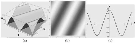
Figure 6. (a)A 3D graph of the periodic soliton solution(3.53)for b=2,ω=0.2,c=2,and-3 ≤t,x ≤3.(b)A 2D density plot of solution(3.53).(c) A 2D graph of solution (3.53) for x=0 and -3 ≤t ≤3.

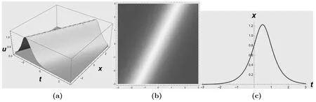
Figure 7. (a) A 3D graph of the bell-shaped soliton solution (3.54) for b=2, c=2,and -3 ≤t, x ≤3.(b) A 2D density plot of solution(3.54).(c) A 2D graph of solution (3.54) for x=1 and -3 ≤t ≤3.

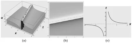
Figure 8. (a) A 3D graph of the singular soliton solution (3.55) for b=2,ω=0.5, c=0.2,and -2 ≤t, x ≤2.(b) A 2D density plot of solution (3.55).(c) A 2D graph of solution (3.55) for t=0 and -2 ≤x ≤2.

Solution set 1.

Solution set 2.

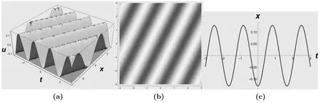
Figure 9. (a)A 3D graph of the periodic soliton solution(3.56)for b=2,ω=0.2,c=2,and-3 ≤t,x ≤3.(b)A 2D density plot of solution(3.56).(c) A 2D graph of solution (3.56) for x=0 and -3 ≤t ≤3.

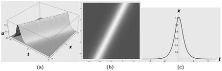
Figure 10. (a) A 3D graph of the bell-shaped soliton solution (3.57) for b=2, c=2,and -5 ≤t, x ≤5.(b) A 2D density plot of solution(3.57).(c) A 2D graph of solution (3.57) for x=0 and -5 ≤t ≤5.

Thus,the dnoidal wave solution of the LGHe (1.3)corresponding to solution set 1 is given by

and for solution set 2 is

The wave profiles of solutions (3.56) and (3.57) are given in figures 9 and 10,respectively.

4.Conservation laws of the LGHe

Conservation laws delineate physical properties that do not change during several processes that take place in the physical world.These quantities are said to be“conserved”.In physics,for instance,the conserved quantities are energy,momentum,and angular momentum.Here,we attain conserved vectors for the LGHe (1.3) via the engagement of two methods.Firstly,the multiplier approach,as shown in [29],and then,the conservation theorem from Ibragimov,given in [56].

4.1.Conservation laws using the multiplier approach

The multiplier approach is admired for its ability to handle conserved quantities of DEs,whether they possess variational principles or not.We employ the multiplier technique to derive conserved vectors for the LGHe (1.3).It is worth noting that the zeroth-order multiplier yields no results;hence,we shall consider first-order multipliers,namely,Λ=Λ(t,x,u,ut,ux),and use these multipliers to establish the conservation laws of equation(1.3).Recall that the first-order multipliers Λ are determined from the determining equation

where δ/δuis the Euler operator given by

By expanding equation(4.58)and following the steps similar to the algorithm for finding the Lie symmetries,we obtain six determining equations,namely,

Solving the above system we get

whereC1,C2,andC3are constants.The required conserved quantities are then found via the divergence identity

whereTtis the conserved density andTxis the spatial flux.Thus,after some tedious computation,the conserved vectors corresponding to the three multipliers are given below.

Case 1.For the first multiplier Λ1=xut+tux,the corresponding conserved vector is given by

Case 2.For the second multiplier Λ2=ux,the corresponding conserved vector is

Case 3.Finally,for the third multiplier Λ3=ut,the corresponding conserved vector is given by

4.2.Conservation laws using Ibragimov’s theorem

The established method states that each symmetry is associated with a specific conserved quantity [56].We now use the conservation theorem from Ibragimov to calculate the conserved vectors of the LGHe (1.3).For a more in-depth understanding of the method,the reader can refer to [56].

The adjoint equation for equation (1.3) can be obtained from the formula

where,v=v(t,x),and this yields

which implies that the LGHe is self-adjoint.Considering equation(1.3)and the adjoint equation(4.62)as a system,the formal Lagrangian for this system is

Recall that the LGHe admits three infinitesimal symmetries.We derive the conserved vectors (Tt,Tx) using the formulae

Case 1.For W1=,the Lie characteristic function is given byW1=-ut.Thus,the conserved vector associated with1W,using equation (4.64),is

Case 2.For the symmetry W2=,the Lie characteristic function isW2=-uxand,consequently,the conserved vector is

Case 3.Finally,for the symmetry W3=,we haveW3=-(tux+xut).Hence,the corresponding conserved vector is

Remarks.Conservation laws play a pivotal role in the analysis of partial differential equations as they provide conserved quantities for the underlying system.These laws not only enable investigations into integrability and linearization,but also have the potential to yield both qualitative and quantitative insights into the properties of the solutions.Among the conserved vectors derived in this study,we have identified those representing linear momentum and energy.Such conserved quantities hold significant value in the examination of physical systems,as they contribute greatly to the understanding of their dynamics and behaviour.Consequently,these conserved vectors offer a valuable framework for studying the intricacies of physical phenomena.Moreover,the conserved vectors involve solutionsuof the LGHe and solutionsvof the adjoint equation(4.62)and,hence,yield an infinite number of conserved vectors.Indeed,it is noteworthy that by settingv=uin the conserved vectors derived using Ibragimov’s theorem,we obtain conserved vectors that closely resemble those obtained through the multiplier method.This observation highlights the connection and similarity between the two approaches in identifying and characterizing conserved quantities in the studied system.It suggests that the multiplier method and Ibragimov’s theorem yield consistent results and provide complementary perspectives on the conservation laws governing the system dynamics.

5.Conclusion

This paper has explored the LGHe from a Lie symmetry perspective.The study has presented a comprehensive account of point symmetries admitted by the LGHe.These symmetries have been utilized to perform symmetry reductions,leading to the discovery of group invariant solutions.Various mathematical tools,including Kudryashov’s method,the extended Jacobi elliptic function expansion method,the power series method,and the simplest equation method,have been applied to obtain solutions characterized by exponential,hyperbolic,and elliptic functions.The presence of arbitrary constants in these solutions enhances their significance and applicability in explaining physical phenomena.To visually represent the obtained solutions,Mathematica was employed to generate 3D,2D,and density plots,as illustrated in figure 1.The plots depict solutions exhibiting kink-shaped,singular kink-shaped,bell-shaped,and periodic patterns.Additionally,the derivation of conserved vectors for the studied model has been accomplished using the multiplier method and Ibragimov’s theorem.This analysis has yielded diverse conserved quantities with practical applications in the field of physical sciences,such as the conservation of energy and momentum.Moreover,among the solutions obtained in this study,only solutions (3.48),(3.50),(3.54),and (3.57)align with the existing literature.However,the remaining solutions are new and novel contributions introduced by this research.Consequently,the newly derived solutions hold potential for further expanding our understanding of the model.

Acknowledgments

M.Y.T.Lephoko would like to thank the South African National Space Agency (SANSA) for funding this work.Additionally,both authors express their gratitude to the Mafikeng campus of North-West University for their ongoing assistance.

Funding

The funding support for this work has been acknowledged.

Conflict of interest

The authors declare that there is no conflict of interest regarding the publication of this paper.

Ethical approval

The authors declare that they have adhered to the ethical standards of research execution.

ORCID iDs

Mduduzi Yolane Thabo Lephokohttps://orcid.org/0000-0001-5407-2956