Planar matrices and arrays of Feynman diagrams: poles for higher k
2024-05-09AlfredoGuevaraandYongZhang
Alfredo Guevara and Yong Zhang
1 Perimeter Institute for Theoretical Physics,Waterloo,ON N2L 2Y5,Canada
2 Department of Physics &Astronomy,University of Waterloo,Waterloo,ON N2L 3G1,Canada
3 Society of Fellows,Harvard University,Cambridge,MA 02138,United States of America
4 CAS Key Laboratory of Theoretical Physics,Institute of Theoretical Physics,Chinese Academy of Sciences,Beijing 100190,China
5 School of Physical Sciences,University of Chinese Academy of Sciences,No.19A Yuquan Road,Beijing 100049,China
Abstract Planar arrays of tree diagrams were introduced as a generalization of Feynman diagrams that enable the computation of biadjoint amplitudes for k>2.In this follow-up work,we investigate the poles of from the perspective of such arrays.For general k,we characterize the underlying polytope as a Flag Complex and propose a computation of the amplitude-based solely on the knowledge of the poles,whose number is drastically less than the number of the full arrays.As an example,we first provide all the poles for the cases(k,n)=(3,7),(3,8),(3,9),(3,10),(4,8)and(4,9)in terms of their planar arrays of degenerate Feynman diagrams.We then implement simple compatibility criteria together with an addition operation between arrays and recover the full collections/arrays for such cases.Along the way,we implement hard and soft kinematical limits,which provide a map between the poles in kinematic space and their combinatoric arrays.We use the operation to give a proof of a previously conjectured combinatorial duality for arrays in(k,n)and(n-k,n).We also outline the relation to boundary maps of the hypersimplex Δk,n and rays in the tropical Grassmannian Tr (k ,n).
Keywords: Feynman diagrams,biadjoint amplitudes,poles
1.Introduction
The Cachazo–He–Yuan (CHY) formulation provides a direct window into the scattering amplitudes of a wide range of Quantum Field Theories,by expressing them as a localized integral over the moduli space of punctures of CP1[1–5].Such formulation was generalized by Cachazo,Early,Mizera,and one of the authors(CEGM),who extended it to configuration spaces over CPk-1,or equivalently to the Grasmanian Gr(k,n)modulo rescalings [6].This unveiled a beautiful connection to tropical geometry,revealing that the CEGM amplitudes (for the generalized biadjoint scalar theory,)can be computed either from a CHY formula or by more geometrical methods[6,7].In particular,the full amplitudecan be obtained as the volume of the positive Tropical Grassmannian TrG+(k,n)viewed as a polyhedral fan.The CEGM amplitudes are also closed related to the cluster algebras [7–16],positroid subdivisions [17–19],and new stringy canonical forms [20–22].The casek=4 is also especially interesting due to its connection with the symbol alphabet of N=4 SYM [8,23–25].
Based on the application of metric tree arrangements for parameterizing TrG(3,n) [26],Borges and Cachazo introduced a diagrammatic description of the biadjoint amplitude,as a sum over such arrangements instead of single Feynman diagrams [27].This was then extended to the casek=4 by Cachazo,Gimenez,and the authors [28]: In this case,the building blocks are not collections but arrays(matrices)of planar Feynman diagrams.Each entry Mijof the matrix is a planar Feynman diagram concerning the canonical ordering {1,…,n}n{i,j}.We endow the diagram Mijwith a tree metricwhich corresponds to the distance between leaveskandlaccording to the diagram Mijand require that it defines a completely symmetric tensor,
The contribution to the biadjoint amplitude is obtained by defining the function
wheresijklare generalized kinematic invariants [6],namely totally symmetric tensors satisfying generalized on-shell conditionsii…=0 and momentum conservation:
Using the Schwinger parametrization of the propagators,identifying Schwinger parameters to the independent internal lengthsfIunder the compatibility constraints (1.1),one can compute the contribution of an array M to the amplitude via
where Δ is the domain whereallinternal lengths are positive.See[27,28]for more details.6The symbolC was used in[28]to denote collections,namely k=3 objects.Here we will respect this notation but further use M to denote both arrays(k=4) and higher rank objects made of Feynman diagram entries.If we define byJ(α)the set of all planar arrays for the ordering α,the biadjoint amplitude for two orderings is then [6]
In this follow-up note,we introduce a new representation of the poles of this amplitude,for the most general caseα=β=In,and also discuss the generalksetup.We then explain how the amplitude can be recovered from such poles when they are understood from planar arrays of Feynman diagrams.This new representation corresponds to collections/arrays of degenerate ordinary Feynman diagrams and can easily be translated to kinematic invariants in terms ofs….This way,we get all the poles for(k,n)=(3,7),(3,8),(3,9),(4,7),(4,8) and (4,9),which agree with those obtained in[21] from the stringy canonical form construction.Conversely,as explained in section 3,we will also explain a method to get all the new presentations of poles as degenerate arrays by applying hard limits to kinematic invariants (in the sense defined in [28,29]).We also provide a map for which any such array defines a ray satisfying tropical Plucker relations and hence lies inside the Tropical Grassmannian polytope TrG(k,n).
In the supplementary data,we provide the explicit degenerate planar arrays for the cases (k,n)=(3,6),(3,7),(3,8),(3,9),(3,10),(4,7),(4,8)and(4,9).Those of(3,10)are obtained by translating the poles given in [21] but one in principle can also get (3,10) planar collections of Feynman diagrams first using the bootstrap method given in [28] and then degenerate them to get all poles in their new representations.
Given two degenerated planar rays V1,V2as poles,we derive and prove criteria to check compatibility in terms of their Feynman diagram components.We show that this criterion can be translated to the weak separation condition studied in the mathematical literature,see e.g.[18,30–32].We then provide an operation of addition which is equivalent to the Minkowski sum of the corresponding tropical vectors.Using this operation we can reconstruct the full facets,e.g.the planar collections and arrays previously obtained in [27,28].More generally we can construct a graph of compatibility relations,where poles correspond to vertices and facets correspond to maximal cliques.This gives a realization of our polytope as a Flag Complex,as observed long ago for the original construction of TrG(3,6)[33].We provide a Mathematica notebook as supplementary data to implement this algorithm for all (k,n) belonging to(3,6)-(3,10) and (4,7)-(4,9).
This paper is organized as follows.In section 2 we construct poles as one-parameter arrays of degenerate Feynman diagrams and explain how to sum them to obtain higher dimensional objects,such as the full arrays of[28].We focus onk=3,4.We then provide the compatibility criteria for generalkand give a Mathematica implementation of the compatibility graphs.In section 3 we present both a kinematic and combinatoric description of the soft and hard limits of the planar arrays of Feynman diagrams.We use it to construct the arrays corresponding to our poles and further prove the general implementation of Grassmannian duality conjectured in[28].In the discussion,we outline future directions as well as a relation with the matroid subdivision of the hypersimplex Δ(k,n).
2.From full arrays to poles and back
Here we initiate the study of higherkpoles from the perspective of collections of tree diagrams.Recall that these correspond to vertices of the dual polytope(up to certain redundancies we will review),or to facets of the positive geometry associated with stringy canonical forms [20].From the perspective of the collections,we shall find that the vertices are,in a precise sense,collections ofk=2 poles.The full collections of cubic diagrams,studied in [28],correspond to convex facets of the (k,n) polytope and can be expressed as (Minkowski) sums of poles.We start the illustration withk=3 and then the general cases.
2.1.k=3 Planar collections,poles and compatibility criteria
An illustrative example is the case of the bipyramidal facet appearing in (3,6) [34].This is ak=3 example but the discussion will readily extend to arbitraryk.The description of the bipyramid in terms of a collection has been done in[27,28].From there,we recall
We denote each planar diagram in the collection vector by,i.e.Cbip=.Note thatdoes not contain theith label.We have labeled byx,y,z,u,v,w>0 six internal distances which are independent solutions to compatibility conditions,
That this collection has the geometry of a bipyramid is seen as follows.We define its six faces by each of the allowed degeneration of metric tree arrangement.These correspond to the hyperplanes
in R4.We can project the planes into three dimensions by imposing an inhomogenous constraint,e.g.x+y+z+w=1,leading to the picture of figure 1.The region where all the distances in (2.1) are strictly positive corresponds to the interior of the bipyramid.The notation for the vertices of the figure,e.g.t1234,t3456,t5612,R,,will become natural in a moment.Two faces that meet at an edge correspond to two simultaneous degenerations.For instance the edge {R,t1234}is given by settingy=0 andz=0,leading to the two-parameter collection:
A vertex is given by three or more simultaneous degenerations.By performing each of the two valid degenerations of the edge,that isx→0 orw→0,we arrive at the following vertices:
We say that two vertices are compatible if they are connected by an edge,which can be either in the boundary or in the interior of a facet.For readers familiar with the notion of tropical hyperplanes,an edge emerges when the sum of the two independent solutions of the tropical hyperplane equations (e.g.two different vertices in TrG) is also a solution,see [7].
Inspection of the facets of (3,6) show that they are all convex and hence any two vertices in a facet are compatible.In the context of planar arrays of Feynman diagrams,we will prove below that this is a general fact for all(k,n).This is also motivated by the original work[33],where it was argued that the polytope (3,6) can be characterized as aFlag Complex,which we can introduce as follows:
Definition 2.1.The Flag Complex associated with a graphGis a simplicial complex (a collection of simplices) such that each simplex is spanned by a maximal collection of pairwise compatible vertices inG.
As a graph,the bipyramid corresponds to a four-dimensional simplex in the sense that it is spanned by the five vertices {R,,t1234,t3456,t5612},which are pairwise compatible,i.e.connected by an edge.However,the edge {R,} is contained inside the bipyramid,which is equivalent to the geometrical fact that the simplex degenerates from four to three dimensions,as we explain below.The three-dimensional object drawn in figure 1 is what we interpret as a facet of the polytope.In general,any simplex of the Flag Complex associated with(k,n)is indeed a geometrical facet,and can be embedded in (k-1)(n-k-1)-1 dimensions.
Following the guidelines from Tropical Geometry it is convenient to interpret each vertex as a ray in the space of metrics embedded in.Explicitly,for a compatible collection (2.2) and a vertex,πijkdepends on a single parameterx>0,and indeed we can write it as a ray πijk∼xVijk.The equivalence ∼here means that we are modding out by the shift
for arbitrarywi.This is a redundancy characteristic of tropical hyperplanes,e.g.[26].7One can also understand this redundancy by realizing Σj,k≠isijkwi=0 on the support of k=3 momentum conservation (2.8),which means the contribution of a planar collection of Feynman diagram to the amplitude like(2.9) keeps the same.An edge then corresponds to the Minkowski sum of two vertices.For instance,the edge {R,t1234} corresponds to a plane ingiven by
We can now justify our notation for the vertices {R,,t1234,t3456,t5612},namely argue for a correspondence between the vertices and kinematic poles.Indeed,the relation(2.7)can be expressed in terms of generalizedk=3 kinematic invariants.Under the support ofk=3 momentum conservation
the ∼symbol turns into an equality:
where we used the definitions
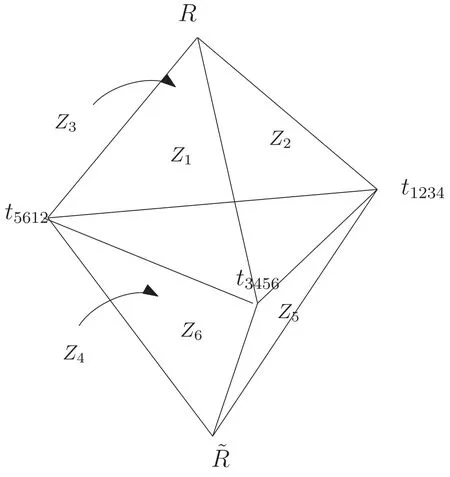
Figure 1. Bipyramid projected into three dimensions.
Assuming that we know the collections (2.5),we can argue that(2.7)indeed defines an edge of the polytope,meaning it is associated with a compatible collection of Feynman diagrams(not necessarily cubic).In other words,we can recover (2.4).Asin (2.7) leads to a fully symmetric tensorby construction,it is only needed to show that this tensor is the metric of a certain collection.This follows from the fact that theith elements ofCRand,sayrespectively,have compatible poles in the sense ofk=2 Feynman diagrams.For instance,has the poles34andhas the poles56,which are compatible.The quartic vertex incan be blown up to accommodate for the poles56and vice versa.As the two diagrams now have the same topology their metrics can be added,thus showing thatis indeed associated with ak=2 Feynman diagram.We depict this in figure 2.Repeating this argument for all the componentsTiwe obtain the following8The ‘only if’ part is easily seen to follow from a known fact of k=2(applied to each of the components Ti): if the sum of two vertices corresponds to a Feynman diagra m (i.e.to a tropical hyperplane or a line in TrG(2,n))then the two vertices VX,VY are compatible as k=2 poles.
Theorem 2.1.Two one-parameter collectionsCX andCY are compatible if and only if their respectivek=2 componentsare compatible for alli.
Now,an important property ofk=2 poles is the following:given a set of poles that are pairwise compatible,e.g.{s12,s123,s56},then such poles are compatiblesimultaneously,meaning that there exists ak=2 Feynman diagram that includes them all.9This is seen as follows: two compatible k=2 poles can be written as sa and sA,where a ⊂A as planar subsets.Another pole that is compatible with sA can be written as sb where b⊂A.As sa and sb are compatible we have either b⊂a, a⊂b or a∩b=∅.In all cases,there exists a Feynman diagram with all three poles.Considering this together with theorem 2.1,we can further state the following
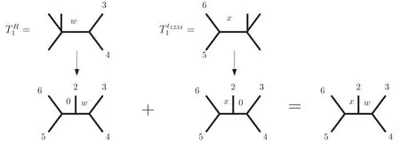
Figure 2.Addition of compatible diagrams.
Corollary 2.1.A set of collectionswhich is pairwisecompatible is also simultaneously compatible.
For collections,simultaneous compatibility means that the Minkowski sum of the corresponding vertices also leads to a collection.This is best explained with our example:using theorem 2.1 we can easily check that the vertices in {R,,t1234,t3456,t5612} are compatible in pairs.This then implies that the Minkowski sum
will also be associated with an arrangement of Feynman diagrams.As we anticipated,this has the topology of a fourdimensional simplex (in a projective sense).However,it degenerates to three dimensions due to the identity
or,in terms of generalized kinematic invariants,
This implies that the Minkowski sum (2.12) can be rewritten as
which indeed lives in three dimensions and spans the bipyramid facet.We can obtain a more familiar parametrization of the facet,as given in [27].First,let us project again the Minkowski sum into kinematic invariants,i.e.
where we have introduced new variables:Because αi>0 we clearly havex,y,z,w>0.Moreover,one can check that two independent linear combinations of the new variables,
are also positive.These are nothing but theu,v>0 conditions that we have started with and recovered our description of the collectionCbip,equation (2.1),whereas F(bipyramid) agrees with that given in[27].Our compatibility criteria thus allowed us to translate back a description in terms of the vertices(2.12)(a Minkowski sum)to a description in terms of the full collection of cubic diagrams.
2.2.Planar arrays and k>3 poles
The previous approach can be extended to the casek>3.Planar arrays of Feynman diagrams fork=4 and higher were defined in [28] as rankk-2 objects,and involve the natural generalization of the compatibility condition (2.2).
Using thesecond bootstrapapproach introduced there,one can obtain matrices of planar cubic Feynman diagrams for(k,n)=(4,7)starting from collections of(k,n)=(3,6).A few interesting features arise for poles ofk=4.Again,let us examine a particular planar array of (4,7) as shown by the symmetric matrix in figure 3 to illustrate the construction of the poles.This array can be obtained from a (3,7) collection via the duality procedure of[28],which we review in the next section.Recall that in this case,the metric compatibility conditions are given by(1.1)and the kinematic function reads
where
together with the corresponding relabelings.Note that for a given columnicompatibility implies
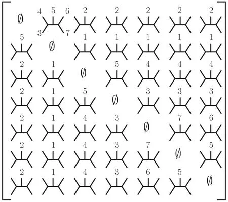
Figure 3.A particular planar array of(4,7).Note that the omitted labels in the Feynman diagram entries can be deduced by their planarity.
hence such a column must be a collection,i.e.corresponds tok=3.For (3,6) such collections can only be bipyramids (as the example of the previous section)or simplices(if they have four boundaries) [33].In fact,for our example,we can write the array Mijas a ‘collection of collections’ as shown in figure 4.
Each entry represents a(3,6)collection,namely a vector of cubic diagrams.They are labeled by kinematic poles as in the previous section,where collectionC(i)contains labels {1,…,7}n{i}.Besides the standard degenerations (boundaries)of eachC(i),we have depicted some internal boundaries in yellow.These arise from the external boundaries of another collection,sayC(j),through the compatibility condition(1.1).For instance,translating the bipyramid boundaries(2.3)to the new variables we used in(2.18)we see that collectionC(5)has the following six boundaries:
which depend only on four variables {x,y,w,q} instead of six,as expected for a bipyramid living in three dimensions.Now,we further consider the following (external)degenerations of collectionsC(1)andC(3),
which altogether induce the planew=yas a new degeneration,depicted by the internal yellow plane bisecting the bipyramidC(5)in (4).The intersection of this plane with its external facesq=q+x-y=0 in (2.22) induces a new ray in (3,6),obtained as the midpoint of the verticest1234andt6712,labelled ast1234+t6712in (4).In the other collectionsC(i),the induced(3,6)rays can be further labeled in the same way and lead to the (4,7) ray we denoteW:
while the kinematic function (2.18) becomes
In(2.23)the sum of vertices must be understood in the sense of the previous section.That is,we consider the line,which belongs to thek=3 polytope sincet6712andt1234are compatible(in fact,they appear together in a bipyramid).The vertext6712+t1234corresponds to its midpointx=y.Addition of (collections of) Feynman diagrams is done as in figure 2,for instance:
where T(i)are rays in (k-1,n-1),which can also be written as arrays of Feynman diagrams.In the previous example this corresponds to our decomposition(2.23),where V(4,7)=MWand T(i)arek=2 rays.
In thek=2 polytope two raysdij(x) andd′ij(y)are compatible (their sum corresponds to a Feynman diagram) if and only if their respective kinematic poles are compatible.which can also be written more compactly as
(Note thats43ands67are compatible,thus their sum also belongs to thek=2 polytope.) Hence each of the entries of(2.23) can be represented as a column,and MWcan be written as a 7×7 matrix with a single internal distance parameterx.This is precisely our original array of cubic diagrams (3) after the degenerations have been imposed.
We have learned that the compatibility condition (1.1) can lead to particular boundary structures as in(2.23).Because of this the vertexWof(4,7)is not only decomposed in terms of vertices of (3,6) but also certain internal rays (midpoints) of the (3,6)polytope.It would be interesting to classify the kind of internal rays that can appear in this decomposition.
2.2.1.Compatibility criteria for general k.We now present the criteria for compatibility of poles,which easily extends from the casek=3 in the previous part of this section to generalk.A vertex of the (k,n) polytope,realized as a ray in the space of metrics will be determined by a completely symmetric array of rankk-2.From now on we will denote such array as,10HereV denotes a generic vertex.For a particular vertex labeled by X,we may use MX as in the previous section.e.g.a vector fork=3 and a matrix fork=4,where each component is a planar Feynman diagram.
Such an array can be organized by ‘columns’ we define by,so we write:
For generalkthis means that the componentsandare compatible if,and only if,the diagramsare compatible in thek=2 sense.Furthermore,two rays represented by arrays V(k,n)and V′(k,n)are compatible when all their diagrams are.This implies the following extension of theorem 2.1
Theorem 2.2.Two vertex arraysV(k,n)andare compatible if and only if their componentsT(i)andarecompatible as rays of(k-1,n-1),for alli=1,…,n.
Assuming we know all possible poles,this provides an efficient criterion for checking their compatibility and,repeating the Minkowski sum construction of the previous section,constructing the facets of the polytope.This criterion has already appeared in the math literature in the context of boundary maps of the hypersimplex Δk,n,see e.g.[18,30,31];11We thank N.Early for pointing this out.we will establish the precise equivalence in section 4.1.
Corollary 2.2.Two vertex arraysV(k,n)andarecompatible if and only if their entriesandare compatible for all{i1,i2,…,ik-2}⊂{1,2,…,n}.
The proof is straightforward.
The full list of poles can be obtained by degenerations of just a few known facets of the polytope,given in our previous work [28],or more simply from singularities in the moduli space through the CPk-1scattering equations of[34],as done in[21].Once the full list of poles is known as a combination of kinematic invariants,we can easily translate them to arrays using the procedure described in the next section.In an attached notebook,we construct the full facets fork=3 andk=4 starting from the kinematic poles and provide a simple implementation of theorems 2.1 and 2.2 to check the compatibility relations of any pair of poles.
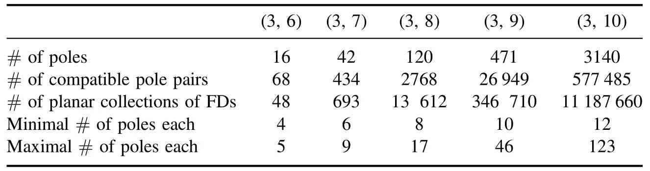
Table 1. The number of poles,pairs of compatible poles,planar collections of Feynman diagrams,and minimal versus maximal number of poles in a single planar collection of Feynman diagrams for k=3.
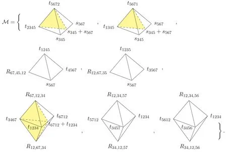
Figure 4.Writing the arrayMij as a ‘collection of collections’.
2.3.Summary of the results
We list the number of poles and the number of pairs of compatible poles for (3,6)-(3,9) and for (4,7)-(4,9) in tables 1 and 2 respectively.What is more,we recover all the planar arrays of Feynman diagrams using the compatibility rules,whose number is also summarized in the tables.Using the(3,10)poles given in[21],we also predict that the number of (3,10) planar collections of Feynman diagrams should be 11 187 660.We see the number of poles is much less than that of planar GFDs.The minimal number of poles for a (k,n)planar array of Feynman diagrams is (k-1)(n-k-1) and we list the maximal number in the tables.We see that a(4,9)planar matrix of Feynman diagrams could have 461 poles,much larger than the minimal number 12.
3.Soft/hard limits and duality
In[29],a kinematic hard limit has been introduced,based on the Grassmannian duality of the generalized amplitudeand its soft limit.Up to the momentum conservation ambiguities,we can define it as (take e.g.particle label 1)
In this section,we give a combinatoric description of such soft and hard kinematic limits in terms of the arrays.This provides a method for constructing the array of a pole only from the knowledge of the corresponding kinematic invariant.
Very nicely,this will also provide a geometric interpretation to the combinatorial soft and hard limits discussed in[28] for facets,e.g.full collections and arrays.At the sametime,it leads to proof of the combinatorial duality proposed there for such facets.
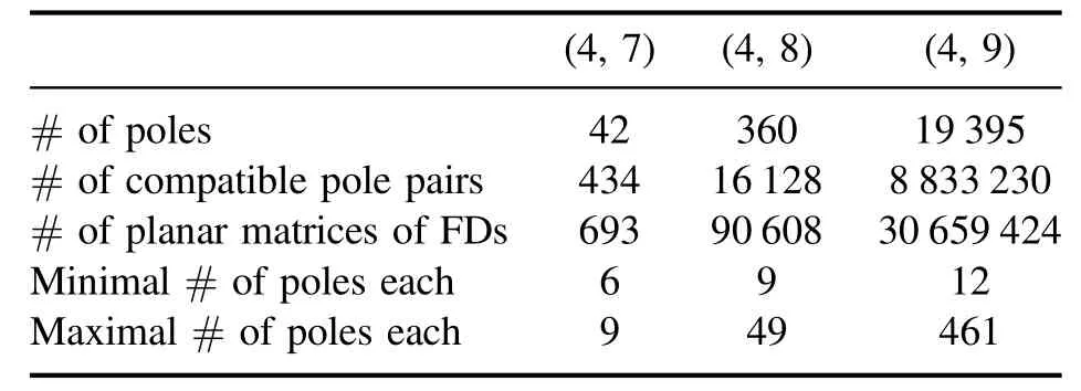
Table 2. The number of poles,pairs of compatible poles,planar matrices of Feynman diagrams,and minimal versus maximal number of poles in a single planar matrix of Feynman diagrams for k=4.
Let us usek=4 as an example to introduce the connection between kinematics and combinatorics.A pole is described in terms of generalized kinematic invariants by the function
Let us first consider the soft limit on label 1,i.e.s1…→extracting the leading order as τ →0.The pole then becomes
The hard limit proceeds in a similar fashion.On label 1,takes1…→and extract the leading terms as τ →∞.The result can be written as
This has a direct application for constructing an array given certain kinematics.Take for instance the poleWin(4,7),equation (2.24)
Under the hard limit in e.g.particle 7
Thus,from(3.4),R12,34,56corresponds to the valuation of the column T(7)in the array ofW,i.e.F (T(7)),and can be used interchangeably.Indeed,by applying the hard limits in all the labels one recovers the array
which justifies the notation (2.23).Of course,each of the elements here is indeed a column,which can be constructed by applying yet another hard limit,e.g.
which is (2.26).Thus,the matrix associated withW1234567is obtained by a consecutive double hard limit.The fact that the matrix (MW)ijobtained so is symmetric corresponds to the statement that the two hard limits commute.
For a general vertex of the (k,n) polytope,of the form(2.27),we have
where T(1)is a vertex of (k-1,n-1) andis a vertex of(k,n-1):
This provides a kinematic interpretation of the combinatorial hard (k-reducing) and soft (k-preserving) operations for generalk,n.Also,givenF (V),the arraycan be constructed by applyingk-2 consecutive hard limits in labelsi1,…,ik-2and identifying the resultingk=2 Mandelstam with a Feynman diagram as in (2.25) and (2.26).
3.1.Duality
It is known that the (k,n) polytope admits a dual description as a (n-k,n) polytope,induced by Grassmannian dualityG(k,n)∼G(n-k,n).In the moduli space,this identification was shown to imply the relation[34,29].In the context of the polytope (i.e.kinematic space),the identification is true for facets,edges,vertices,etc.Indeed,a duality for planar arrays of Feynman diagrams was conjectured in[28]and relates arrays in(k,n)and(n-k,n).It is such that
under appropriate relabeling.Furthermore,both collections M(k,n)and M*(n-k,n)have the same boundaries arising as degenerations and hence lead to the same contribution to the biadjoint amplitude.
We now describe and provide a proof of the duality.Let us first consider the case of vertices and then promote it to facets via the sum procedure of the previous section.Two vertices in (k,n)and (n-k,n)are defined as duals when they satisfy
i.e.they are kinematically the same.
Of course,the previous definition requires relabeling the kinematic invariants.Focusing on the case (4,7)∼(3,7) to illustrate this,the relabeling issabcd∼sefgwhere{a,b,c,d,e,f,g}={1,…,7}.Suppose nowa=1.The hard limit in label 1 ofs1bcd
while under the soft limit
But {b,c,d,e,f,g}={2,…,7} and hence~sefgunder the duality (3,6)∼(3,6).This can be repeated while replacings1bcdby any linear combination of kinematic invariants,in particular by the one given byF (V).The conclusion can be nicely depicted by the diagram:
But from (3.9) we conclude that F (T(1))~.That is,the (k-1,n-1)arrayT(1),which is the first column ofV,is dual to the (n-k,n-1) array,which corresponds toV*with the first components removed.Repeating the steps for all other labels proves the following:
Theorem 3.1.LetV*(n-k,n)be the dual ray toV(k,n)=[T(1),…,T(n)],that isF (V)=F (V *)under appropriaterelabelings.Then the hard limitT(i)is dual to the soft limitfor alli=1,…,n.
Since soft and hard limits always reduce the number of labelsn,this theorem can be iterated to check whether two given rays are duals.
This criterion was conjectured for facets in [28].To prove the criteria for two dual facets,say M(k,n)and M*(n-k,n),we resort to the construction in section 2.According to the characterization 2.1 of the polytope,facets or full collections are maximal sums of poles.Using the notation of equation (2.12) for the space of compatible metrics for an array,we can write
or simply,using the addition of compatible Feynman diagrams
Now let us define the following object:
The duality relation (3.11) follows from (3.12) together with the linearity of the mapF.Of course,this definition requires that the verticesV*Ican be added.We now prove
Theorem 3.2.The set{V *Iis a maximally compatiblecollection of vertices(a clique)of(n-k,n).HenceM*is afacet,the dual facet ofM.
Proof.It suffices to show that if two vertices,say V and W,are compatible,so are their duals V* and W*.This follows from induction inn(the casen=4 being trivial):If V and W are compatible in (k,n),it is easy to see that their combinatorial soft limitsare compatible in(k,n-1),for alli.Then,using the induction hypothesis we find that their duals,are compatible.From theorem 3.1 these are the hard limits of V* and W* for alli.It then follows from theorem 2.2 that V* and W* are themselves compatible as(k-n,n)arrays,which completes the induction. □
Having successfully characterized the dual facet of M by equation (3.18) we can now prove the extension of theorem 3.1 for facets.For this,let us simply denote bythe combinatorial soft limit of M in particlei,which indeed defines a facet of the (k,n-1) polytope.From (3.17),it is easy to see that the soft limit is
On the other hand the combinatorial hard limit of M*(given by (3.18)) in particleiis
4.Discussion
In [28],a combinatorial bootstrap was introduced for obtaining the collections corresponding to facets of(k,n)withk≥4.In a nutshell,fork=4 one writes a candidate symmetric array of Feynman diagrams using as a set of columns the facets of (3,n-1),i.e.
Then,one checks whether the corresponding metriccan be imposed to be symmetric,in which case a facet of(4,n)is found.In this work,we have explored the representation(4.1)for vertices V of (k,n).However,in section 2.2 we have discovered that in this case the columns T(i)(which play the role of theCiin (4.1)) are not necessarily vertices of(k-1,n-1) but rather certain internal rays in the polytope.It would be interesting to classify which kind of internal rays can appear,as a way of implementing the combinatorial bootstrap more efficiently at the level of vertices.Interestingly,for all the examples explored in this work,we were able to check a weaker version: a compatible collectionfor which all theare vertices in (k-1,n-1) is indeed a vertex of (k,n).For instance,for (4,8) we obtain 98 poles given by all possible compatible collections of poles of (3,7) (also including the trivial column).
Despite these subtleties,we found there is a universal way to translate any poles in terms of generalized kinematics as degenerated arrays and vice versa,check their compatibility relations,and reconstruct the full planar arrays of Feynman diagrams for anyk≥3.
This research opens up a myriad of intriguing mathematical avenues for further investigation.Primarily,our exploration in this paper delves into the poles of the partial amplitudein alignment with the concept of global planarity.Notably,in [35,36],there is the introduction of diverse forms of partial amplitudes grounded in the idea of local planarity.This encompasses the usage of generalized color orderings to elaborate on the color-dressed generalized biadjoint amplitudes.An exciting prospect would be the application of our current methodology to probe into these broader partial amplitudes,emphasizing their poles manifested as degenerate arrays and their ensuing compatibility criteria.
Since the initial unveiling of CEGM amplitudes in [6],the field has witnessed considerable advancements.Prominent among these are the exploration of generalized soft theorems[29,37],the discernment of the semi-locally triple splitting amplitudes [38],and the unveiling of certain factorization channels [39,40].Furthermore,comprehensive characterizations of the scattering equations have been presented in [34,41–45] within the original CEGM integrals in configuration spaces over CPk-1.Delving into the intricate relationships between the poles and these inherent properties of the amplitudes promises to be a captivating avenue of research.
Our findings also suggest potential intersections with positroid subdivisions [17–19],intricate combinatorial structures that provide a richer context to the dynamics of the amplitudes.Let us end up this paper by a brief discussion on the relation between the higherkpoles to boundary map from the (k,n) hypersimplex.This offers an intriguing perspective that may act as a stepping stone for subsequent inquiries in this domain.
4.1.Relation to boundary map from the (k,n) hypersimplex
The hard limit we have introduced here can be understood as a map (k,n)→(k-1,n-1) for any ray in TrG(k,n).Early introduced a basis of planar poles,corresponding to certain matroid subdivisions of the hypersimplex Δ(k,n)[18,19,32].Then,there is a natural boundary restriction ∂(j)Δk,n=Δk-1,n-1that can be applied to characterize such matroid subdivisions.When acting on Early’s planar basis,we will now argue that the boundary restriction agrees with our hard kinematical limit.Since the action of the boundary restriction on a generic pole is the linear extension of the action on the basis,this means that the hard limit effectively implements the boundary map in general.
We construct the planar basis as follows: consider the hypersimplex Δk,ndefined by
LetI⊂{1,…,n} be a subset ofkelements,|I|=k.The vertexeI∊Rnof the hypersimplex corresponds toxi=1 fori∊I,with all the otherxl=0.The boundary ∂(j)Δk,nis obtained by settingxj=1,i.e.it becomes the hypersimplex Δk-1,n-1given by Σi≠jxi=k-1.Note that this decreases the value ofkandnexactly as the hard limit introduced in section 3.Focusing on the boundaryx1=1,let us denote its vertices bywhere⊂{2,…,n}with=k-1.
Positroid subdivisions can be obtained from the level functionh(x):Δk,n→Rstudied in [18,19].This is piecewise linear in the hypersimplex and its curvature is localized on certain hyperplanes defining the subdivision.Early’s basis is in correspondence with the subdivisions arising in the set of functions
Since there arenconsecutive subsetsI,the number of such functions is-n,precisely the number of independent kinematics for (k,n).12In this notation a set of independent kinematic invariants (which is nonplanar,i.e.does not entirely correspond to the poles of ,is generated by sJ with |J|=k.Recall that we further have n momentum conservation constraints,in this notation =0 for all j=1,…,n.To obtain the explicit planar basis in kinematic space we take the linear combination(up to an overall normalization)
(One can check that by virtue of momentum conservation ηJ=0 for a consecutive subsetJ[18]).Now we show that the hard limit as constructed in section 3 has precisely the same effect as the boundary map restriction ∂(1)of the subdivisionh(x-eJ).Taking the hard limit in label 1 we obtain:
Recall that the hard limitsare interpreted here as the kinematic invariants for(k-1,n-1),i.e.a system that does not include particle label 1.From (4.5) we conclude that the functionh(x-eJ) that defines de subdivision is restricted to the domainx∊∂(1)Δk,nafter the hard limit is taken.Hence the boundary restriction of the subdivision is equivalent to the hard limit on the basis ηJ,as we wanted to show.
Very nicely,the hard limit of ηJalso gives an element of the planar basisfor (k-1,n-1).For instance,ifJis of the formJ=,it clear from (4.5) that we obtain.A similar analysis can be done for generalJand recovers the general rule given in[18]for the boundary map.
A future direction is to further elucidate the relation between the compatibility formulation using Steinman relations/Weak Separation[18,19]and the compatibility criteria implemented here in the context of planar arrays of degenerate Feynman diagrams.
Acknowledgments
We thank F Cachazo and B Gimenez for their collaboration in the initial stages of this project.We would like to thank F Cachazo and N Early for the useful discussions.Research at the Perimeter Institute is supported in part by the Government of Canada through the Department of Innovation,Science and Economic Development Canada and by the Province of Ontario through the Ministry of Economic Development,Job Creation and Trade.
杂志排行

Communications in Theoretical Physics的其它文章
- Diffusion of nanochannel-confined knot along a tensioned polymer*
- Study of scalar particles through the Klein–Gordon equation under rainbow gravity effects in Bonnor–Melvin-Lambda space-time
- Holographic dark energy in non-conserved gravity theory
- Phase structures and critical behavior of rational non-linear electrodynamics Anti de Sitter black holes in Rastall gravity
- Two-component dimers of ultracold atoms with center-of-mass-momentum dependent interactions
- Electrical characteristics of a fractionalorder 3 × n Fan network