Research on Flexible Job Shop Scheduling Based on Improved Two-Layer Optimization Algorithm

Qinhui Liu,Laizheng Zhu,Zhijie Gao,Jilong Wang and Jiang Li

College of Mechanical and Electrical Engineering,Harbin Engineering University,Harbin,150001,China

ABSTRACT To improve the productivity,the resource utilization and reduce the production cost of flexible job shops,this paper designs an improved two-layer optimization algorithm for the dual-resource scheduling optimization problem of flexible job shop considering workpiece batching.Firstly,a mathematical model is established to minimize the maximum completion time.Secondly,an improved two-layer optimization algorithm is designed: the outer layer algorithm uses an improved PSO(Particle Swarm Optimization)to solve the workpiece batching problem,and the inner layer algorithm uses an improved GA (Genetic Algorithm) to solve the dual-resource scheduling problem.Then,a rescheduling method is designed to solve the task disturbance problem,represented by machine failures,occurring in the workshop production process.Finally,the superiority and effectiveness of the improved two-layer optimization algorithm are verified by two typical cases.The case results show that the improved twolayer optimization algorithm increases the average productivity by 7.44% compared to the ordinary two-layer optimization algorithm.By setting the different numbers of AGVs (Automated Guided Vehicles) and analyzing the impact on the production cycle of the whole order,this paper uses two indicators,the maximum completion time decreasing rate and the average AGV load time,to obtain the optimal number of AGVs,which saves the cost of production while ensuring the production efficiency.This research combines the solved problem with the real production process,which improves the productivity and reduces the production cost of the flexible job shop,and provides new ideas for the subsequent research.

KEYWORDS Dual resource scheduling;workpiece batching;rescheduling;particle swarm optimization;genetic algorithm

1 Introduction

With the increasing automatic level in the manufacturing industry and the constant changes in market demand,it is necessary to improve manufacturing flexibility and resource utilization,as well as reduce the production cycle to meet the gradually formed market demand characterized by multi-variety,small batch,product customization and short production cycle [1].The production mode of manufacturing enterprises has also shifted from the traditional special line production to the flexible multi-variety and small batch mixed-flow production mode [2].The flexible workshop,which combines the advantages of traditional production run and flexible production,can fit the product variety,differentiated mixed line production well,and it has become a mainstream mode that manufacturing enterprises use to deal with multi-variety and small batch mixed line production [3],especially in the military,aerospace,automotive fields.

In the flexible production mode,most parts are processed and transferred according to a certain batch size,except for some large or special equipment parts that need to be produced in a single piece[4].AGVs are widely used in the production process of flexible workshops to complete the transfer task of parts in the production process because of their automation,high efficiency and flexibility[5].The quality of the workpiece batching and the transfer efficiency of AGVs will have a great impact on the job shop scheduling.Therefore,the flexible job shop scheduling problem considering AGV transportation and workpiece batching constraints has certain theoretical significance and engineering application value.

Flexible Job Shop Scheduling Problem (FJSP) is an extension of the Job Shop Scheduling Problem (JSP),which breaks through the limitation of JSP that each process is machined only on one determined machine tool.For FJSP,each process can be machined on multiple optional machine tools[6],which is more in line with actual production needs.Research on FJSP has generally focused on solving the problem of machine optimal scheduling,i.e.,choosing a reasonable processing machine for each process of each workpiece and formulating a reasonable processing sequence to optimize production[7,8].However,most studies of FJSP scheduling optimization are mainly based on singlepiece scheduling[9–11],ignoring the fact that the flow and transportation process of the workpieces among different processes and the machining and transshipment processes of most parts are carried out according to a certain batch in the flexible production mode,which is not in line with the actual production process.

In summary,although FJSP can solve sub-problems such as process sequencing and machine selection in a way that a certain batch of workpieces is regarded as a whole,the division of the batch in production has a greater impact on optimization objectives such as the completion time[12].Therefore,the study of the workpiece batch scheduling problem of the flexible job shop is of great significance in guiding the actual production and improving the utilization of machine tools.This problem is more complex than the traditional FJSP,and the solution should not only consider process sequencing,machine selection but also consider batch division including the number of batches and the batch size of each sub-batch[13].The job shop scheduling problem considering workpiece batching has received academic attention in recent years;however,the overall research is relatively scarce.Wang et al.[14]proposed the Hybrid Particle Swarm Algorithm to solve the batch scheduling problem in solar cell manufacturing,stating that machine allocation,batch determination and production sequencing for each batch were linked and needed to be jointly optimized.Low et al.[15] demonstrated that batch scheduling of workpieces could improve productivity and solved the common batch scheduling problem in production.Sun et al.[16]proposed the Genetic Algorithm for batch scheduling workpieces in equal quantities,which could optimize the batch division and the machining order of sub-batches simultaneously.Yan et al.[17]used the PSO and the improved PSO to solve the variable batch flow shop problem.And this result showed that the improved PSO increased the range,depth and speed of particle search;therefore,the optimal solution capability and stability of the improved PSO were better than the standard PSO and other methods.Although the above studies have achieved some results in batch division,they have neglected the link between the batch requirements of the product and the dual resource(machine tools and AGVs)constraints.

Integrating machine tools with AGVs for scheduling will speed up the material flow and improve the production management efficiency of the workshop.Therefore,more and more scholars are starting to integrate AGVs and machine tools for scheduling.In the research of dual-resource scheduling problems,most scholars use intelligent algorithms to solve them.Liu et al.[18]established a mathematical model of dual-resource scheduling containing machine tools and AGVs for the problem of segment AGV flexible job shop scheduling optimization.They designed an improved genetic algorithm to solve the problem and verified the superiority of the algorithm through a standard case.Zhu et al.[19]studied flexible job shop scheduling containing AGVs to minimize the maximum completion time.They proposed an improved genetic algorithm and compared it with two classical heuristic algorithms in experiments to verify the feasibility and effectiveness of the new algorithm.Sanches et al.[20]proposed to use an adaptive GA to solve the scheduling problem when considering the simultaneous use of machines and AGVs to minimize the manufacturing cycle time.They verified the computational results in larger scenarios and compared the adaptive GA with other methods,which obtained better results.However,the above studies only consider the static constraints of machine tools and AGVs,ignoring the fact that dynamic abnormal disturbance events will inevitably occur during the actual production process,such as equipment failures,emergency order insertion,delivery time changes and other uncertain disturbance factors [21],which affects the reliable and stable operation of the production system.And these uncertainties have a greater impact on the original production plan and even cause the scheduling program formulated in advance to be no longer effective.With the continuous application of IoT information technology in the production process,such as sensors,machine vision,etc.,the relevant information in workshop production can be sensed in real-time by a series of intelligent workshop devices[22].These technological means can summarize and analyze the real-time production data to help the enterprise to master the real-time production status of the workshop in order to prevent the impact of the dynamic abnormal disturbance events on the production in advance,so the study of the flexible job shop rescheduling is of great significance.

Therefore,this paper designs an improved two-layer optimization algorithm for the dual-resource scheduling optimization problem of flexible job shops considering workpiece batching to minimize the maximum completion time.The outer algorithm uses the improved PSO to solve the workpiece batching problem and uses the obtained workpiece batching scheme as an input to the inner algorithm.The inner layer algorithm uses an improved GA to solve the dual-resource scheduling problem.Moreover,a rescheduling method is designed for disturbance events during the production process.The effectiveness of the two-layer optimization algorithm is verified by a typical case.The impacts of different numbers of AGVs on the production process are analyzed,and the optimal number of AGVs is determined by the maximum completion time decreasing rate index.

The contributions of this paper to the dual resource scheduling optimization problem of flexible job shop considering workpiece batching are as follows:

1.For the dual-resource scheduling optimization problem of flexible job shop considering workpiece batching,a dual-resource scheduling optimization model considering workpiece batching is established to minimize the maximum completion time.

2.Combining the advantages of PSO and GA,this paper designs an improved two-layer optimization algorithm to solve the dual-resource scheduling problem considering workpiece batching.For the outer algorithm PSO,it is improved by using linearly decreasing inertia weights,time-varying acceleration factors,etc.For the inner algorithm GA,a three-layer coding method is designed,and the Hill-Climbing strategy,the hybrid selection strategy of roulette and tournament,adaptive crossover,adaptive variation and other improve methods are also added.The case results show that compared to the ordinary two-layer optimization algorithm,the improved two-layer optimization algorithm takes less time and has a higher average productivity in solving the dual-resource scheduling optimization problem for flexible job shop considering workpiece batching.

3.Due to the uncertainty of the scheduling environment,some abnormal events may occur in real industry production,which may cause the initial scheduling scheme to be unexecuted.This paper takes the failure of processing equipments as the disturbance event,and designs a rescheduling method.The simulation results of the test case show that a better result can be achieved,which is more in line with the real production process.

The other parts of the work are as follows:

Section 2 describes and analyzes the dual-resource scheduling optimization problem of flexible job shop considering workpieces batching and constructs a mathematical optimization model;Section 3 designs an improved two-layer optimization algorithm for solving the dual-resource scheduling optimization problem of flexible job shop considering workpieces batching;Section 4 verifies the validity of the algorithm through a typical case study,and gives a recommendation on the number of AGVs;Section 5 summarizes and discusses the research content of this paper.

2 Problem Description and Modeling

The dual-resource scheduling optimization problem of flexible job shop considering workpiece batching can be described as:

When a flexible job shop is performing a production task,there arentypes of workpiecesJ={J1,J2,...,Jn},which need to be processed onmmachine toolsM={M1,M2,...,Mm};there arekAGVs that are responsible for the workpiece transfer taskV={V1,V2,...,Vk};each type of workpiece is divided into a certain number of production batchB={B1,B2,...,Bn};each sub-batch of production will be taken as a whole for the transfer and processing task;each workpiece has at least one process and each process can choose any machine tool that meets the machining requirements.

Assumptions:

1.Each production sub-batch is transported and processed as a whole;

2.Different production sub-batches can be processed in parallel without being subject to the process sequence constraint;

3.Only one production sub-batch can be processed on one machine tool at the same time;

4.After the machine tool has started machining,the process cannot be interrupted unless there is a malfunction in that machine tool;

5.All machine tools have unlimited material buffer capacity,and only one AGV can be parked at a time;

6.The AGV travels at a constant speed,independent of its unloaded and loaded transportation status;

7.The AGV shall not be interrupted during the transfer of workpieces unless there is a conflict or malfunction;

8.The machining process does not take into account switching times for different workpieces in the same production sub-batch;

9.The installing material time and the removing material time of the machine tools are included in the corresponding machining time;

10.The installing material time and the removing material time of the AGVs are included in the corresponding transportation time;

11.In the initial state,the workpiece rough is in the warehouse,and the AGVs are parked at the outbound platform in the warehouse;

12.No consideration of the AGV power constraint.

To facilitate the establishment of the mathematical model,according to the above assumptions,the introduced parameter symbols and decision variables are defined in Table 1.

Table 1: Symbols and their definitions

Decision variables:

where,i,f=1,2,...,n;q,h=1,2,...,NOi;c=1,2,...,m;a=1,2,...,k;j,g=1,2,...,Bi.

Objectivefunction:

where,denotes the one with the largest completion time among all types of workpieces.

Constraint conditions:

Eq.(6)represents the workpiece batch constraint,i.e.,the number of workpieces in any production sub-batch should be less than or equal to the minimum value of both the AGV’s single maximum load capacity and the total number of workpieces in that category.And the number of workpieces in any production sub-batch should be greater than one.Eq.(7)indicates that the sum of workpieces in the different sub-batches after workpiece batching should be equal to the total number of workpieces of that type.Eq.(8)indicates that only one production sub-batch can be processed on one machine tool at the same time.Eq.(9)indicates that a process in any production sub-batch can only be machined on one machine tool at the same time.Eq.(10)indicates that one AGV can only transfer workpieces of one production sub-batch at the same time.Eq.(11)indicates that the workpieces of any production subbatch can be only transferred by one AGV at the same time.Eq.(12)represents the process start time constraint,i.e.,the start processing time of any process should be greater than or equal to the maximum value of both the end time of the AGV loaded transferring the process and the end time of the current machine tool processing the previous task.Eq.(13) represents the AGV loaded transfer start time constraint,i.e.,the start time of any process of the AGV’s load transfer should be greater than or equal to the maximum value of both the unload end time of the AGV and the end time of the previous process.Eq.(14) represents the machine tool selection constraint,i.e.,any process must choose a machine tool from the set of available machine tools.Eq.(15)represents the process constraints,i.e.,any workpiece can be added to the next process only after its current process is completed.Eq.(16)indicates that the machine tool is not allowed to be interrupted during machining.Eq.(17)indicates that the AGV is not allowed to be interrupted during the transfer task.Eq.(18)represents the delivery period constraint,i.e.,the maximum completion time cannot exceed the delivery period.

3 Design of Improved Two-Layer Optimization Algorithm

In this section,an improved two-layer optimization algorithm is designed to solve the dualresource scheduling optimization problem of flexible job shop considering workpiece batching by combining the advantages of the PSO and the GA.The outer layer algorithm adopts the improved PSO to solve the workpiece batching problem,and the inner layer adopts the improved GA to solve the dual resource scheduling problem.The basic solution flowchart of the improved two-layer optimization algorithm is shown in Fig.1.

3.1 Design of Outer Layer Batch Optimization Algorithm

The outer layer algorithm in this paper uses the PSO to solve the problem of workpiece batching.And the solved workpiece batching scheme is used as the input to the inner layer dual-resource scheduling algorithm to solve the dual-resource scheduling scheme under this batching scheme.Then the fitness of the dual-resource scheduling scheme solved by the inner layer algorithm is used as the fitness of the outer layer algorithm to evaluate the quality of that batching scheme.

Commonly used heuristic optimization algorithms include intelligent optimization algorithms such as the Simulated Annealing(SA),the GA,and the PSO.The principle of the PSO is simple and easy to implement,and fewer parameters need to be adjusted.The PSO also has fast convergence and high efficiency.The outer layer batch optimization algorithm is based on the PSO for solving,but the algorithm’s global search ability is relatively poor,and it is easy to fall into the local optimum[23,24].Therefore,the PSO is improved as follows.

Each particleiin PSO algorithm contains a D-dimensional velocity vectorvij=[vi1,vi2,...,viD]and a position vectorxij=[xi1,xi2,...,xiD],and in each round of iterations,the particle continuously updates its position and velocity by two optimal values.The equations for updating the velocity and position of a particle are shown in Eqs.(19)and(20).

where,vijis the velocity vector;xijis the position vector;tis the number of current evolutionary generations;ωis the inertia weight;c1andc2are the individual learning factor and the group learning factor,respectively;r1andr2are random numbers between[0,1].

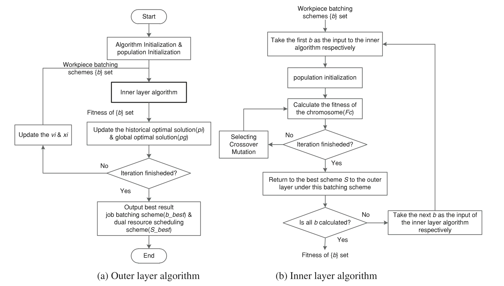
Figure 1:Flow chart of dual-resource batch scheduling optimization in flexible job shop

This paper refers to the linearly decreasing inertia weights proposed by Shi et al.[25]to improveω.The aim is to enable the algorithm to search globally as much as possible in the early iteration and gradually converge to a better local region to conduct a finer search at a later stage,thus finding the global optimal solution.The improved inertia weighting formula is shown in Eq.(21).In addition,this paper refers to the time-varying acceleration factor proposed by Ratnaweera et al.[26]to improvec1andc2in the algorithm.In the early iteration of the algorithm,setting a largerc1and a smallerc2allows individuals to traverse the entire search space and does not converge to the local optimal region quickly;while in the late iteration of the algorithm,a smallerc1and a largerc2,can motivate the particles to converge to the global optimal region.The improved learning factor calculation formulas are shown in Eqs.(22)and(23).

where,Kis the total number of evolutionary generations;ωtis the corresponding inertia weight of the current number of evolutionary generations;ωsis the initial inertia weight of the algorithm,ωeis the final inertia weight of the algorithm,generally based on experience:ωs=0.9,ωe=0.4.

where,c1sandc2sare respectively the initial values ofc1andc2;c1eandc2eare respectively the final values ofc1andc2,generally based on experience:c1s=c2s=0.5,c1e=c2e=2.

In this paper,the workpiece batching method uses the equal batching principle under the relevant constraints of Eqs.(6)–(18).For workpieces of typeawith a total production volumeNJathat is a composite number,equalization of batches must be possible;However for workpieces withNJathat is a prime number,it is not possible to equalize the batches accurately.Therefore,this paper uses the following method for approximation:Firstly,theNJaof the workpiece is subtracted by one to obtain the idealizedNJa.Secondly,the equal batch operation is carried out following the idealizedNJato obtain all the divisible batch numbersBithat can be divided by the idealizedNJa.For the different divisible batch numbers,one of the production sub-batches is randomly selected to be added one to satisfy the actual total production of the workpieces.The basic solution flow is shown in Fig.2.

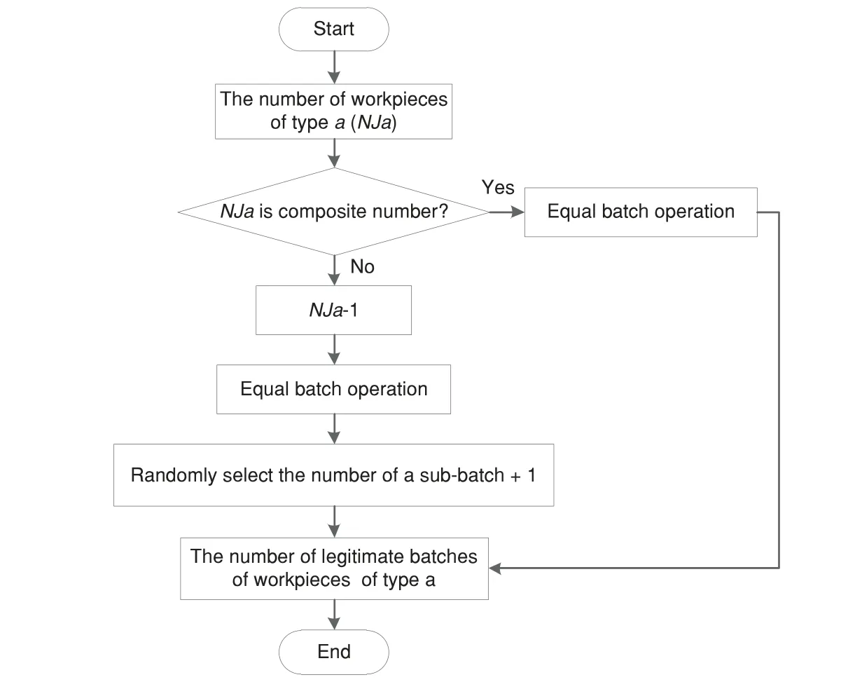
Figure 2:Flow chart of workpiece batching method

The specific steps of the outer layer improved particle swarm algorithm for solving the workpiece batching scheme are as follows:

Step 1:Initialize the total number of evolutionary generationsKand the population sizeNof the outer layer algorithm.Calculate the number of legal batches into whichntypes of workpieces can be divided.

Step 2:Set the current evolutionary generationt=1,and randomly initialize the velocityviand positionxiof all particlesiaccording to the number of legal batches,where the initial positionxiof each particleiforms the setBof the initial workpiece batching scheme.

Step 3:Sequentially take the workpiece batching schemes[b1,b2,...,bn]from setBas the inputs to the inner layer dual-resource scheduling algorithm,and use the fitnessF(xi)of the best dual-resource scheduling scheme searched under each workpiece batching scheme as the fitness of that workpiece batching scheme.

Step 4:Update the historical optimal solutionpi=[pi1,pi2,...,pin] for each particleiand the global optimal solutionpg=[pg1,pg2,...,pgn]for the population.

Step 5:Check whether the termination condition of the algorithmt=Kis satisfied.If so,output the optimal workpiece batching schemesbbest=[b1_best,b2_best,...,bn_best] and the dual-resource scheduling schemeS,and the algorithm iteration is finished;otherwise,go toStep 6.

Step 6:Within the legal search space,updateviandxiaccording to Eqs.(19)–(23).

Step 7:The updated workpiece batching schemes[b1,b2,...,bn]are all passed into the inner layer dual-resource scheduling algorithm andF(xi)is computed by calling the inner layer algorithm.

Step 8:Go toStep 4and performt++.

3.2 Design of Inner Lay Dual-Resource Scheduling Algorithm

The inner dual resource scheduling algorithm is based on the GA because it has strong global search ability,and the GA is easy to combine with other algorithms,which can solve nonlinear and discontinuous problems.However,the GA coding and decoding are more complex,slower convergence,and the GA is more dependent on the initial population [27,28].Therefore,the dual resource scheduling scheme is solved by the improved GA in this section,as follows.

3.2.1 Encoding

Each chromosome is encoded in three layers:the Order Select(OS)layer,the Machine Select(MS)layer,and the AGV Select(AS)layer.

The OS layer adopts decimal coding.The specific coding rule for each gene of the chromosome is in the form of “a.b”,where a indicates the workpiece number and b indicates the batch number.The times that a number appears on the chromosome indicates the total number of processes of the workpiece.The order in which the numbers appear indicates the corresponding processes.All processes of all workpieces from different batches are randomly combined into a complete OS layer chromosome.As shown in Fig.3,if a chromosome sequence contains 12 genes{a1,a2,...,a12},the first occurrence of the number “2.1”on the gene a1means “Workpiece 2 Batch 1 Process 1”,and the decimal “2.1”occurs three times,meaning that“Workpiece 2 Batch 1”has three processes,and so on.

Figure 3:Example of the OS layer coding scheme

MS layer adopts integer coding mode,and the chromosome length of MS layer is the same as the OS layer.The numbers on each gene represent the machine tools of the corresponding process.MS layer coding mode is shown in Fig.4: the three processes of the number “workpiece 1 batch 1”on the first three genes of the chromosome choose machine tool 2,machine tool 5,and machine tool 6,respectively.And so on,we can get the selected machine tools for all the processes of all the workpieces of different batches.

Figure 4:Example of the MS layer coding scheme

The AS layer uses integer coding,and each of its genes corresponds to the OS layer one by one.The AS layer coding is shown in Fig.5.The number“2”on the genea1indicates“Workpiece 2 Batch 1”,which chooses AGV No.2 to perform the transfer task,and so on,to obtain the AGV selection scheme for all processes.

Figure 5:Example of the AS layer coding scheme

3.2.2 Population Initialization

To improve the quality of the initial population of the genetic algorithm and maintain the diversity of the population,this paper designs different initialization methods for the three-layer coding method.The OS layer chromosomes are first initialized through a completely random way,and then further optimized using the Hill-Climbing Algorithm,which effectively improve the quality of the initial solution and the convergence speed of the algorithm.

The MS layer chromosomes are initialized through a combination of a random selection strategy and a global selection strategy,where the random selection ensures the diversity of the population and improves the global search capability of the algorithm,and the global selection strategy ensures the load balancing of the machine tool.

The AS layer chromosomes are initialized by a random method firstly.However,the task allocation to AGVs during the scheduling process is based on the principles of first-come-first-served and load-balancing,which specifically means that when there is an idle state AGV waiting for a task to be allocated,the AGV closest to the task node is selected to perform the transported task;when there is no idle AGV waiting to be allocated,the task is batched to the AGV with the shortest cumulative load time.

3.2.3 Selection

The Roulette Selection Method allows lower fitness individuals to have some probability of being selected,maintaining population diversity to some extent.Tournament Selection is a method of choosing better-adapted individuals to the next generation based on random selection,thus increasing the probability of good genes being passed on in the population.This paper adopts a mixed selection strategy of the roulette selection and the tournament selection to choose half the size of the population individuals,respectively.

3.2.4 Crossover

The OS layer chromosomes and the AS layer chromosomes use Precedence Operation Crossover(POX),as shown in the Fig.6.The MS layer uses Multi-point Crossover (MPX),as shown in the Fig.7.

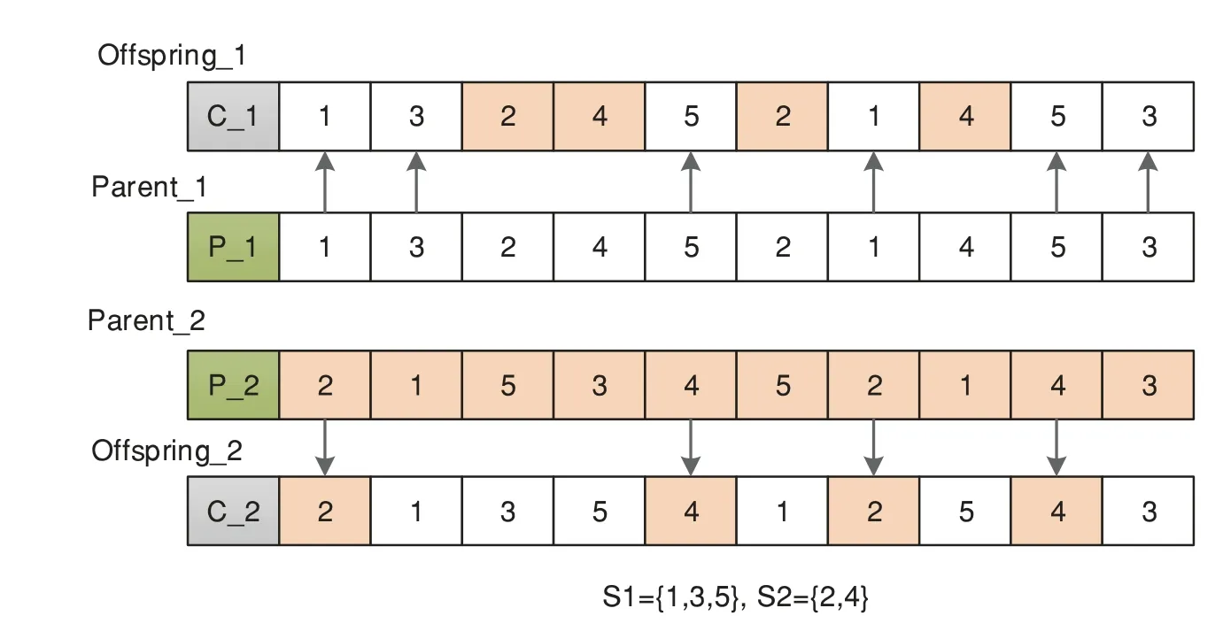
Figure 6:POX crossover process

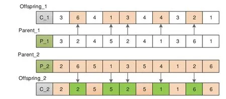
Figure 7:MPX crossover process

Whether a chromosome crosses over is related to the size of the crossover probabilityPc.Too largePcmay lead to the breakage of good individuals in the population;too smallPcleads to a reduction in the convergence speed of the algorithm and in the global search capability[29].In this paper,adaptive crossover probability is used,which is calculated as shown in Eq.(24).

where,fmaxis the largest fitness of all individuals in the population;favgis the average fitness of all individuals in the population;fbigis the larger fitness of the two individuals to be crossed;Pc1andPc2are the crossover parameters,generally based on experience:Pc1=0.9,Pc2=0.6.

3.2.5 Variation

Both the OS and AS layers of the chromosome use the reciprocal variation operation,as shown in Fig.8.The gene position is randomly selected on the MS layer chromosome and its corresponding workpiece number and process number are determined,and then one other machine tool is randomly selected to replace the current machine tool from machine collection of this process,as shown in Fig.9.

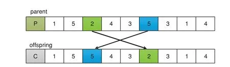
Figure 8:Interchange mutation operation

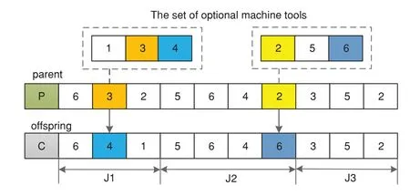
Figure 9:Multi-point mutation operation

When setting the mutation probabilityPm,ifPmis too large,the genetic algorithm will be similar to the ordinary random search algorithm,thus losing its meaning;however,ifPmis too small,it is not easy to generate new individuals,which may cause the algorithm to fall into the local optimal solution during the search process[29].This paper uses the adaptive mutation probability to solve the above problem,and the calculation formula is shown as Eq.(25).

where,Pm1andPm2are the variation parameters,generally based on experience:Pm1=0.1,Pm2=0.01.

3.2.6 Selection of Parameters

The selection of parameters for the GA and the PSO algorithm has an impact on many factors,such as the accuracy and speed of the algorithm and relates to the quality of the results and system performance[30,31].Therefore,it is necessary to analyze the parameters in the two-layer optimization algorithm.

Since the evolutionary generationKand population sizeNhave a large impact on the solution performance of the improved two-layer optimization algorithm in this paper,these two parameters need to be adjusted according to the actual situation during the optimization process.The solution is unstable ifKis too small,and the optimization process is very time-consuming ifKis too large.The smallerNis easy to fall into the local optimum;the largerNcan improve convergence and find the global optimal solution faster,but the computational amount of each iteration will also increase accordingly.Moreover,whenNincreases to a certain level,continuing to increaseNwill no longer have a significant effect.The following paper discusses the sensitivity ofKandN.

3.3 Design of Rescheduling Method Based on Disturbance Events

The scheduling process in a manufacturing shop is full of uncertainties,such as machine failures,emergency order insertions,etc.[32].By timely triggering rescheduling to generate a new scheduling program,the production plan is adjusted according to the new program to ensure the stability of production process.In this paper,the disturbance event takes machine failure as an example.

3.3.1 Rescheduling Strategy

Rescheduling consists of two main aspects:one is the time of starting a new round of scheduling,and the other is the method used for the new round of scheduling.In the application case of this paper,the strategy of rescheduling is to start a new round of scheduling immediately when the disturbance event occurs.You et al.[33]introduced the sequential deviation and completion time deviation as the rescheduling evaluation indexes to choose from the two rescheduling methods-right-shift rescheduling and complete rescheduling.In terms of all aspects of the indexes,the performance of the scheme obtained from complete rescheduling is better.In this paper,the rescheduling method adopts the complete rescheduling method,i.e.,in a new round of scheduling,all the current unfinished workpieces are included in the object set of this scheduling.

When a sudden equipment failure occurs,according to the state of each workpiece and each process in the set of processing objects,the object of rescheduling will be reestablished.According to the processing state,the workpieces and the working processes are divided into three categories:completed processes,processing processes and waiting for processing processes.The processes that are interrupted by equipment failures,as well as the processes of newly arrived workpieces are added to the set of waiting for processing processes.The rescheduling object is the set of processes that are being processed and those that are waiting to be processed,and the information about the idle moments of the equipment is updated at the same time.

3.3.2 Rescheduling Process

Before the disturbance event occurs,the workpiece information and equipment information are known and will not be changed.The processing of the product is executed according to the initial scheduling plan until all workpieces have been processed.When a disturbance event occurs,a rescheduling operation is performed according to the processing status of each workpiece and the status of each piece of equipment.The rescheduling process is shown in Fig.10.

4 Case Studies

This section initially compares the improved two-layer optimization algorithm with the ordinary two-layer optimization algorithm through a case in Section 4.1,and verifies the superiority of the improved two-layer optimization algorithm of this paper through the solution results.Then,a new case is added in Section 4.2,and the outputs of the two cases are obtained to mutually corroborate the effectiveness of the algorithm.

4.1 Algorithmic Superiority Verification

4.1.1 Description of Case 1

The production demand of a production case is 6 kinds of workpieces(J1–J6).The number of each kind of workpiece is shown in Table 2.The process flow data of each workpiece is shown in Table 3,where the data indicates the machining time of the process on the corresponding machine tools and the“—”indicates that the process cannot be processed on the corresponding machine tools.The distance between the workshop machine tools,the warehouses and the individual machines is shown in Fig.11.There are 8 machine tools involved in this case (M1–M8),where: the blue nodes are machine tools;the yellow nodes are warehouses;the number between each node indicates the distance between the nodes.In addition,a total of 4 AGVs perform the workpiece transfer task:the transportation speed is 30 m/min,and the single load capacity is 10 workpiece.

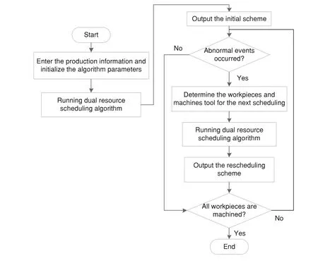
Figure 10:Rescheduling process

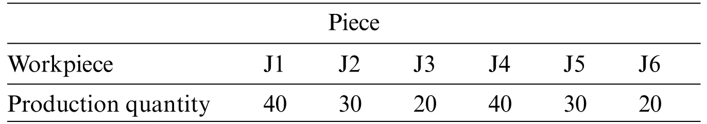
Table 2: The production batch of each workpiece of case 1

Table 3: Workpiece process flow of case 1

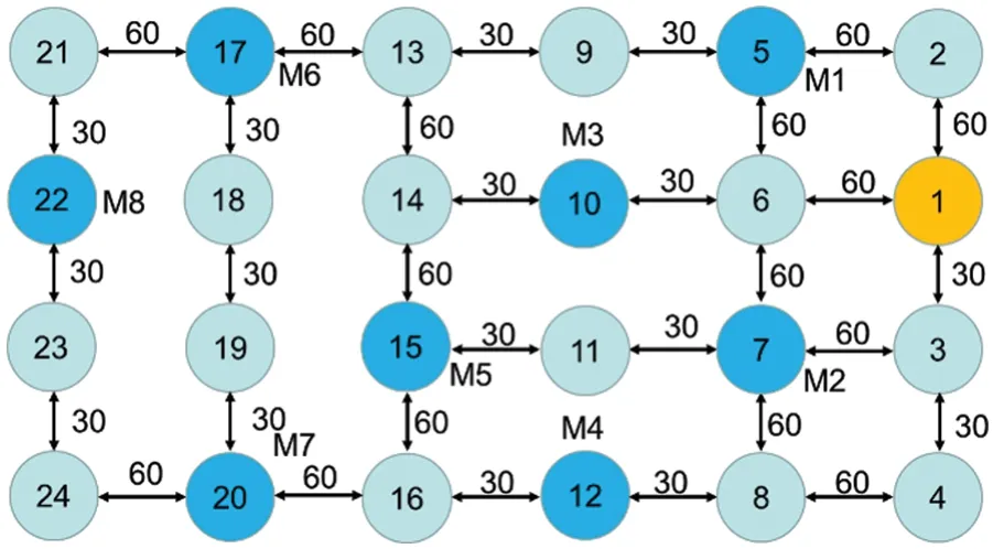
Figure 11:Electronic map of workshop

4.1.2 Parameter Sensitivity Analysis

SinceKandNhave an enormous impact on the solution performance of the improved twolayer optimization algorithm in this paper,a sensitivity analysis of these two important parameters is conducted here.To analyze the parameterK,Nis set to 50 and other parameters keep constant using the control variable method.The above case is solved by setting differentK.Different values ofKare calculated 10 times,and then,the average of the calculated results is analyzed.The results of the experimental statistics are shown in Fig.12.The experimental results show that whenKis set too small,the global optimal solution cannot be searched;whenKis set to 100,the algorithm can search for the global optimal solution in the solution space,but continuing to increaseKwill only increase the computation time of the algorithm and will not search for a better solution.Therefore,the optimalKsetting in this paper is 100.

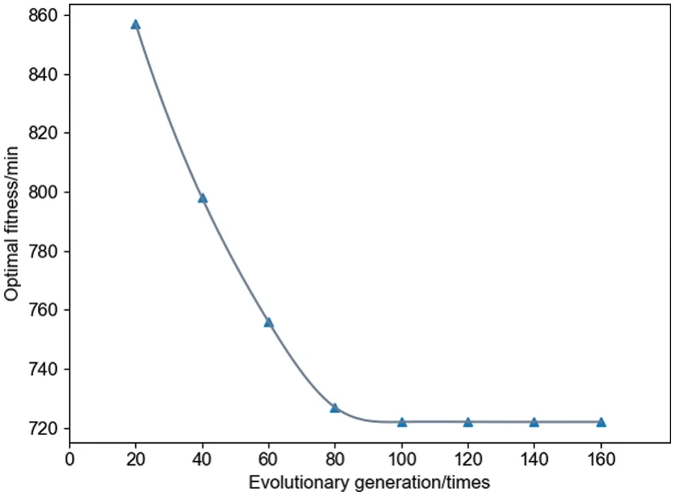
Figure 12:Effect of the K on the optimal fitness

To analyze the parameterN,Kis set to 100 and other parameters keep constant using the control variable method.The above case is solved by setting differentN.The experimental results are shown in Fig.13.The experimental results show that the global search ability of the algorithm increases asNincreases;However,whenNexceeds 50,the global optimal solution searched remains stable asNcontinues to increase,only that the number of evolutionary generations of the algorithm decreases.Therefore,the optimalNin this paper is 50.

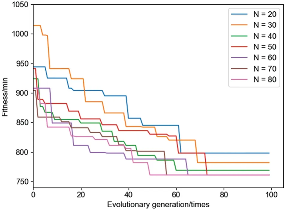
Figure 13:Effect of the N on the optimal fitness

4.1.3 Algorithm Comparison

In the same configuration environment,the above case is solved by the improved two-layer optimization algorithm and the ordinary two-layer optimization algorithm,respectively.

The outer layer of the ordinary two-layer optimization algorithm uses the traditional PSO algorithm with particle updating just following Eqs.(19)–(20),whereas the improved PSO algorithm has particle updating using Eqs.(19)–(23) for each of the parameters.The inner layer algorithm of the ordinary optimization algorithm adopts the traditional GA algorithm,which uses a completely randomized method to generate the initial population for the OS,MS and AS layers in the initialization stage of the population.However,the improved two-layer algorithm in this paper designs different initialization methods for the three layers of coding methods,where the OS layer is initialized by a completely randomized method first and then further optimized by a hill-climbing algorithm,and the MS and AS layers are initialized by a combination of a random selection strategy and a global selection strategy.The ordinary optimization algorithm only uses roulette selection in the selection phase,and the improved two-layer algorithm uses a hybrid selection strategy of roulette selection and tournament selection to select individuals of half the population size separately.The crossover and variation of the ordinary optimization algorithm are randomized without using Eqs.(24)and(25),where:thec1andc2in the ordinary two-layer optimization algorithm are both set to 2;ωis set to 0.9;PcandPmare set to 0.9 and 0.05,respectively;Kis set to 100 andNis set to 50 in both algorithms.The rest of the parameters are the same.According to the production information of the above case,10 calculations are carried out,respectively.The results comparison is shown in Fig.14.The iteration curve of the optimal fitness is shown in Fig.15.

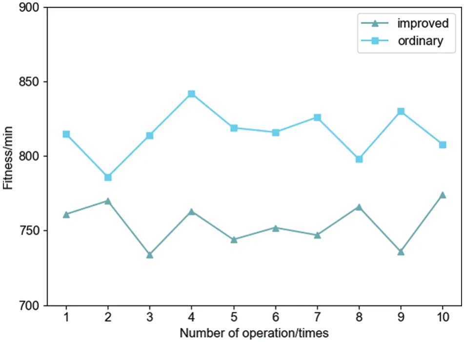
Figure 14:Comparison of the optimal fitness of the two algorithms running 10 times

The solution results of the above two algorithms show that the minimum value of the optimal solution of the improved two-layer algorithm for 10 runs is 734 min,while the minimum value of the optimal solution of the ordinary two-layer optimization algorithm is 786 min,which is an increase in productivity of 6.62%.The average value of the optimal solution of the improved two-layer optimization algorithm is 754.7 min,while the average value of the optimal solution of the ordinary two-layer algorithm is 815.4 min,which is an increase in the average productivity of 7.44%.Since the ordinary two-layer optimization algorithm is easy to fall into the local optimal solution in the iteration process,its solution effect is relatively poor.

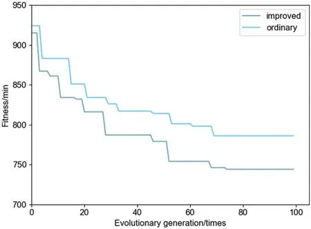
Figure 15:Curves of the optimal fitness for the two algorithms

4.2 Algorithmic Effectiveness Verification

To prove the validity of the algorithm and the model,and to solve case 1 and case 2 simultaneously,the operation results of improved two-layer optimization algorithm in different cases are given to verify each other.

4.2.1 Description of Case 2

The production requirements for case 2 are shown in Table 4;the process flow data for each workpiece is shown in Table 5;the e-map still uses Fig.10,and the number between each node indicates the distance between nodes.In this case,there are three AGV workpiece transfer tasks,all with a speed of 30 m/min and a single load capacity of 10 pieces.

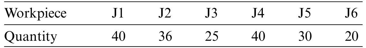
Table 4: The production batch of each workpiece of case 2

Table 5: Workpiece process flow of case 2

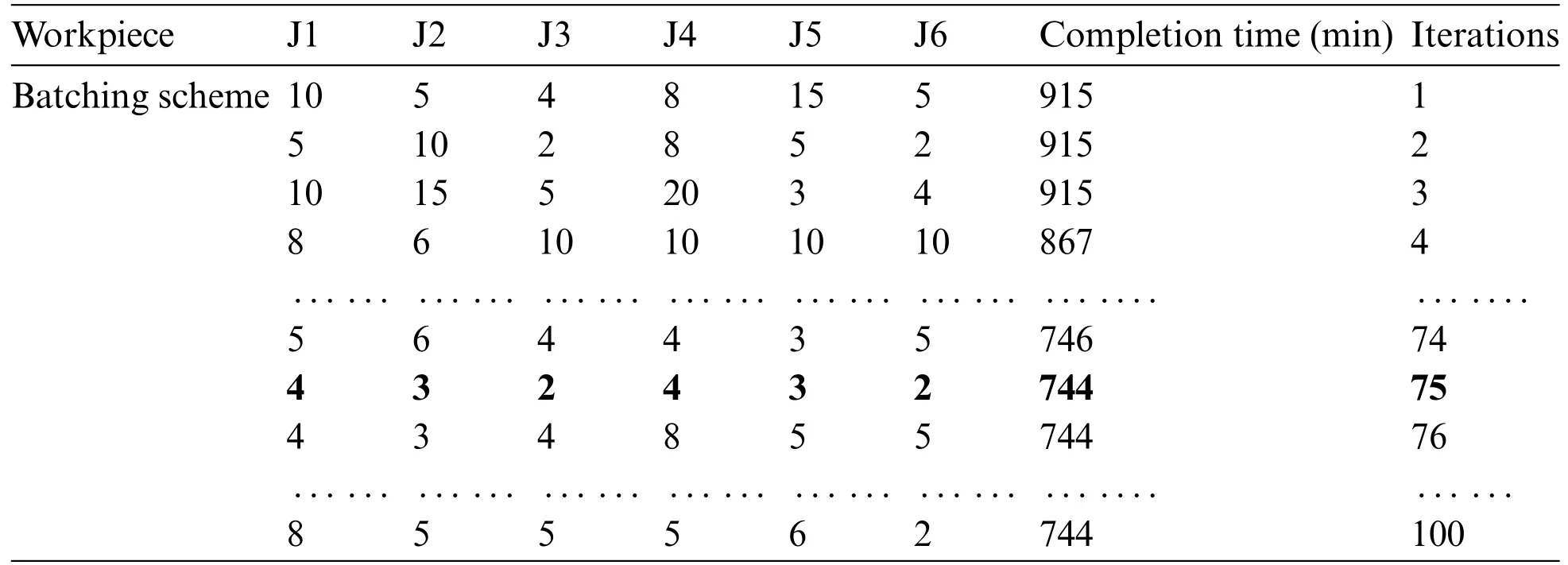
Table 6: Iterative results of the batch optimization scheme of case 1

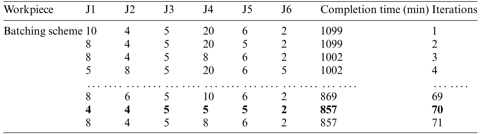
Table 7: Iterative results of the batch optimization scheme of case 2

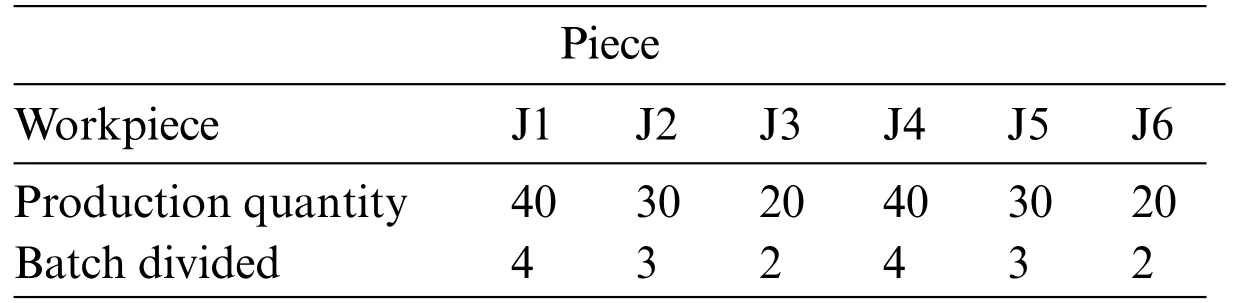
Table 8: Optimal workpiece batching scheme of case 1

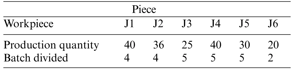
Table 9: Optimal workpiece batching scheme of case 2

4.2.2 Scheme Demonstration

With minimizing the maximum completion time as the objective function,the improved two-layer algorithm designed in this paper is used to solve case 1 and case 2,where the number of evolutionary generations is set to 100 and the population size is set to 50.The iterative curves of the algorithm are shown in Fig.16.The batching information of the solution process is shown in Tables 6 and 7.The optimal workpiece batching scheme is shown in Tables 8 and 9.The optimal dual-resource scheduling scheme is shown in Figs.17 and 18,where:the rectangles of different colors in the Gantt chart represent different workpieces;the numbers on top of the rectangle blocks indicate the batch number;the sequence of the same workpieces appearing in the same batch indicates the process order.

Fig.19 shows the machine working time and AGV working time for case 1 and case 2,respectively,where the machine working time is the cumulative machining time of the workpiece,and the AGV working time is the AGV load traveling time.Meanwhile,both skewness and kurtosis are used to evaluate machine processing time,AGV load time and the load balancing of them.

Figure 16:Curves of the algorithm iteration

In statistics,Skewness can be used to measure the asymmetry of the probability distribution of a random variable and is calculated as Eq.(26).When the value of Skewness is close to 0,it means that the data is relatively evenly distributed on both sides of the average value,indicating a more even distribution.Kurtosis measures the kurtosis of the probability distribution of a real random variable and is calculated as Eq.(27).A Kurtosis above 3 indicates a relatively sharp distribution of data,and a Kurtosis below 3 indicates a relatively flat distribution of data.During the calculation,Kurtosis is usually subtracted by 3 to adjust the kurtosis of the normal distribution to 0,i.e.,a Kurtosis of less than 0 indicates that the data are more average.

where,is the average value of the data;sis the standard deviation of the data;ndis the sample size of the data.After calculation,Skml_case1≈0.084,Kuml_case1≈-1.439 andSkml_case2≈0.340,Kuml_case2≈-0.404 for the machine load time.SkAl_case1≈-0.857,KuAl_case1≈-0.864 andSkAl_case2≈-1.500,KuAl_case2≈-0.172 are for the AGV load time.The resulting data distribution is relatively symmetrical and more balanced.

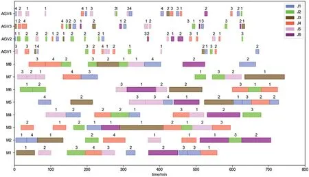
Figure 17:Dual-resource scheduling gantt chart of case 1

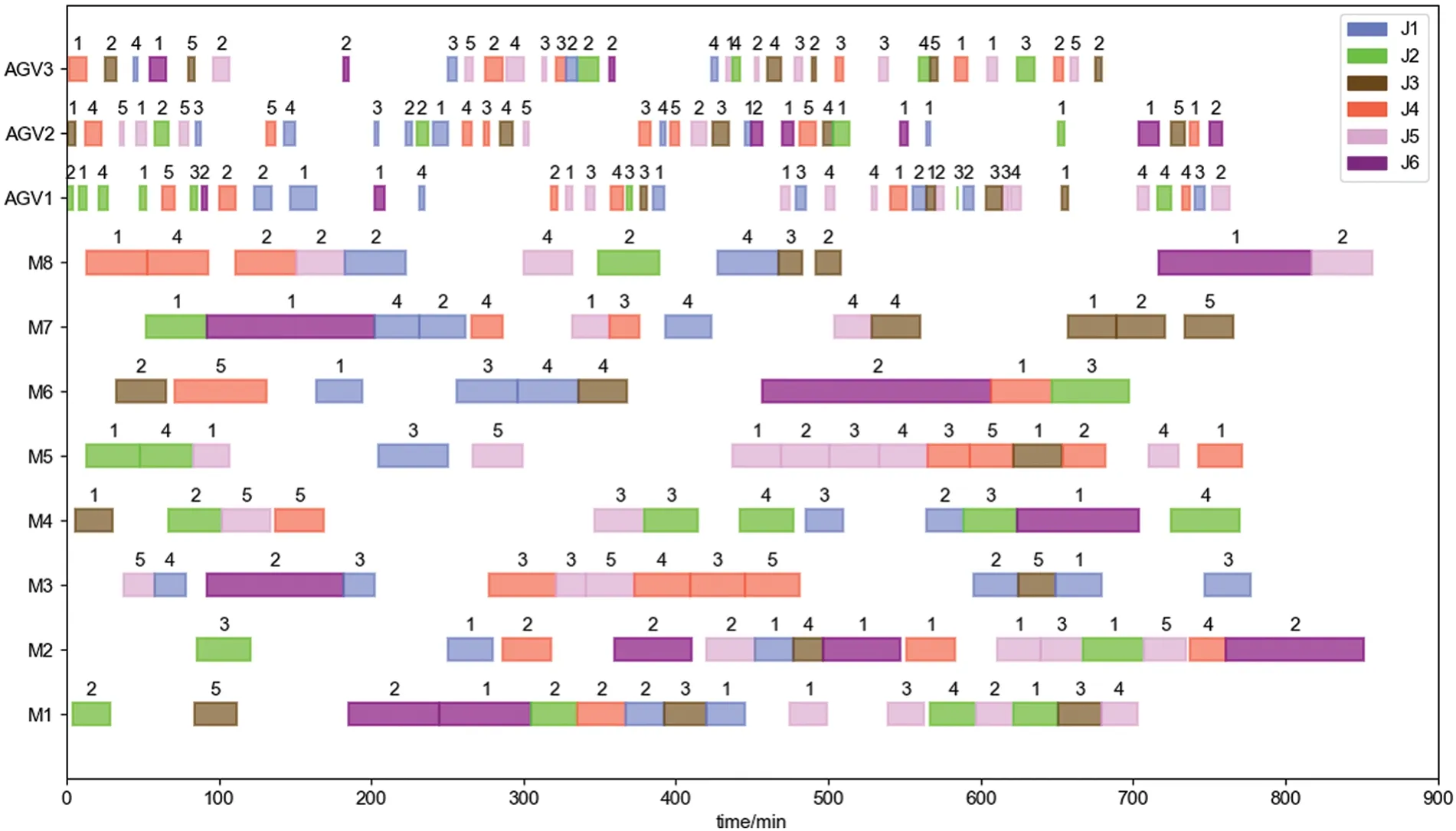
Figure 18:Dual-resource scheduling gantt chart of case 2

4.2.3 Demonstration of Rescheduling Scheme

To verify the performance of the algorithm in solving the rescheduling schemes,it is assumed that machine tool 3 fails at 500 min on case 1 and 400 min on case 2 in the production process of the workshop,and both the required repair time is 50 min.The Gantt chart of the system after the rescheduling is shown in Figs.20 and 21,where the two black dashed lines indicate the start and end time of the failure,and the black rectangle in between indicates the repair time of the faulty machine tool.

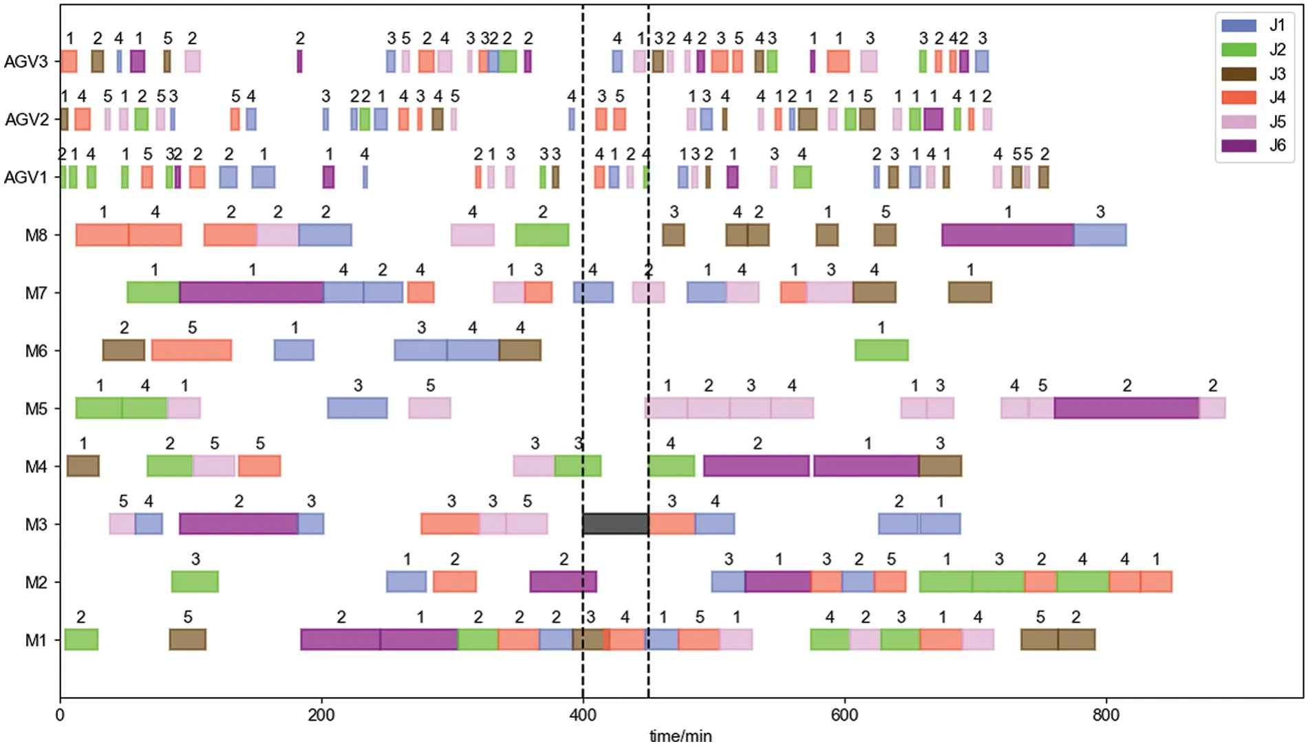
Figure 21:Rescheduling gantt charts of case 2

From the above discussion and result analysis,it can be concluded that the improved two-layer optimization algorithm designed in this paper can effectively solve the dual-resource scheduling optimization problem of flexible job shop considering workpiece batching,and the solution effect is significantly better than the ordinary two-layer optimization algorithm.In addition,the algorithm and rescheduling strategy designed in this paper can deal with the abnormal disturbance events in a timely and effective manner and obtain good rescheduling results.

4.3 AGV Quantity Analysis

In the actual operation environment of the workshop,although increasing the number of AGVs can directly improve the operational efficiency,too many AGVs will cause themselves to wait for each other,which will easily cause congestion in the transportation area.Therefore,reducing the number of AGVs under the requirement of meeting the task time can effectively reduce the congestion of AGVs and the probability of waiting for each other[34].On the other hand,as the number of AGVs increases,the cost is increasing.Therefore,determining a reasonable number of AGVs under the premise of meeting the processing requirements is of great significance in reducing the congestion and the cost of AGVs.

To explore the number of AGVs,an actual production case is analyzed below.There are 6 types of workpieces to be processed in the case.The production batch of each type of workpiece is shown in Table 10.The process of workpiece machining flow is shown in Table 11.The electronic map of the workshop equipment layout is shown in Fig.10.

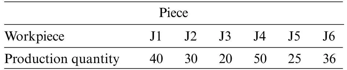
Table 10: The production batch of each workpiece

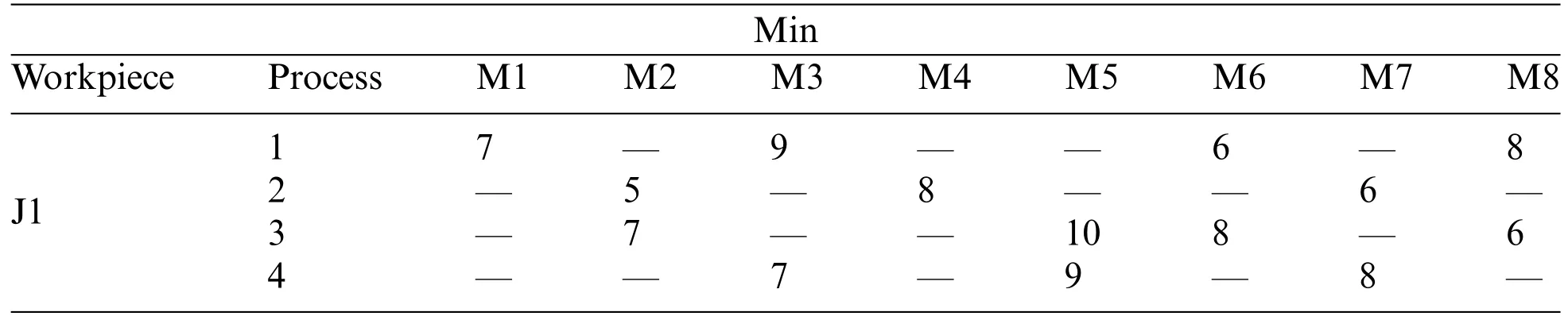
Table 11: Workpiece process flow

There are 8 machine tools in the workshop.The traveling speed of AGV is 25 m/min,and the maximum single load capacity is 10 pieces.The number of AGVs is changed sequentially from 1–8 by the enumeration method,and the best scheduling scheme under this number of AGVs is obtained by iterative optimization of the algorithm.The maximum completion time decreasing rate [35] and the average AGV load time are used as evaluation indexes for the optimal number of AGVs,and the formulas for both are Eqs.(28)and(29).

where,Tagvdenotes the average AGV load time;Rddenotes the maximum completion time decreasing rate;kdenotes the number of AGVs;Akdenotes the load time of thekthAGV,i=1,2...k;Tkdenotes the maximum completion time ofkAGVs.

The above case is solved using the improved two-layer optimization algorithm designed in this paper with minimizing the maximum completion time as the objective function.The algorithm’sKis set to 100 and N is set to 50.The optimal workpiece batching scheme is obtained as shown in Table 12.The optimal solution iteration curves,the effect on maximum completion time are shown in Fig.22.The effect on maximum completion time decreasing rate,and the effect on average AGV load time at different numbers of AGVs are shown in Fig.23.Figs.24–27 respectively show the Gantt charts of the optimal dual-resource scheduling scheme for the cases with the number of AGV configurations of 2,4,6,and 8.

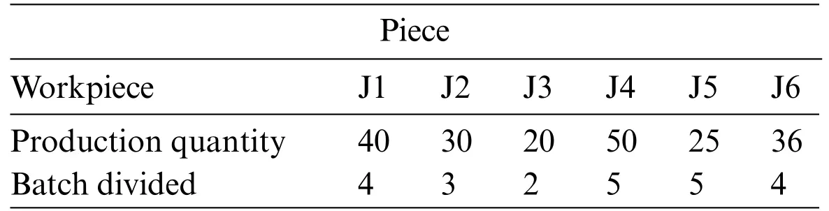
Table 12: Optimal workpiece batching scheme

The results are analyzed as follows:From Fig.22,it can be seen that when the number of AGVs exceeds 6,the increase in the number of AGVs has very little effect on reducing the maximum completion time.This is because the idle time and the path waiting time of AGVs keep increasing with the increase in the number of AGVs,while other conditions remain constant.From Fig.23,it can be seen that when the number of AGVs exceeds 6,RdandTagvof the AVG is very small as the number of AGVs increases.Taken together,the optimal number of AGVs for this case is 6.

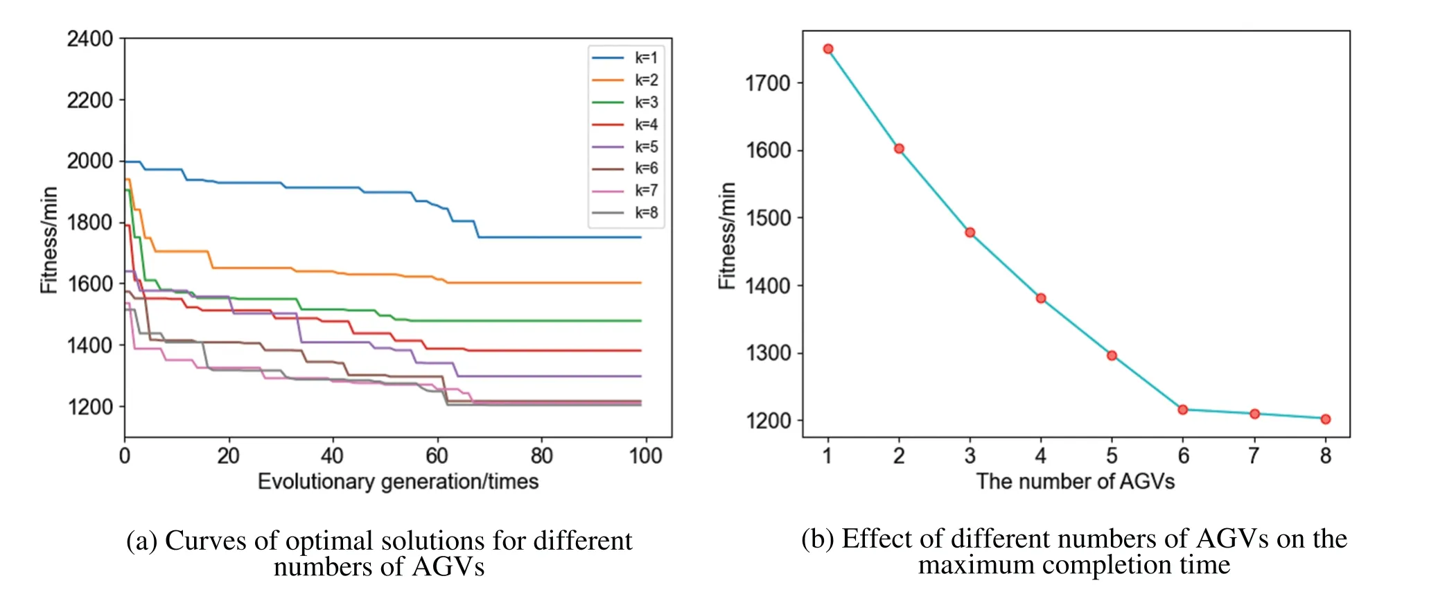
Figure 22:Simulation results of algorithm performance

Figure 23:Effect of different numbers of AGVs on Rd and Tagv

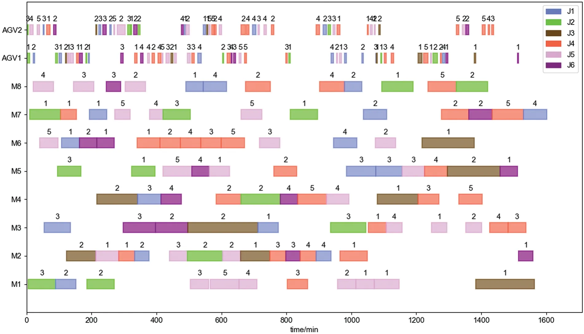
Figure 24:Scheduling scheme with 2 AGVs

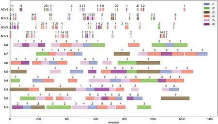
Figure 25:Scheduling scheme with 4 AGVs

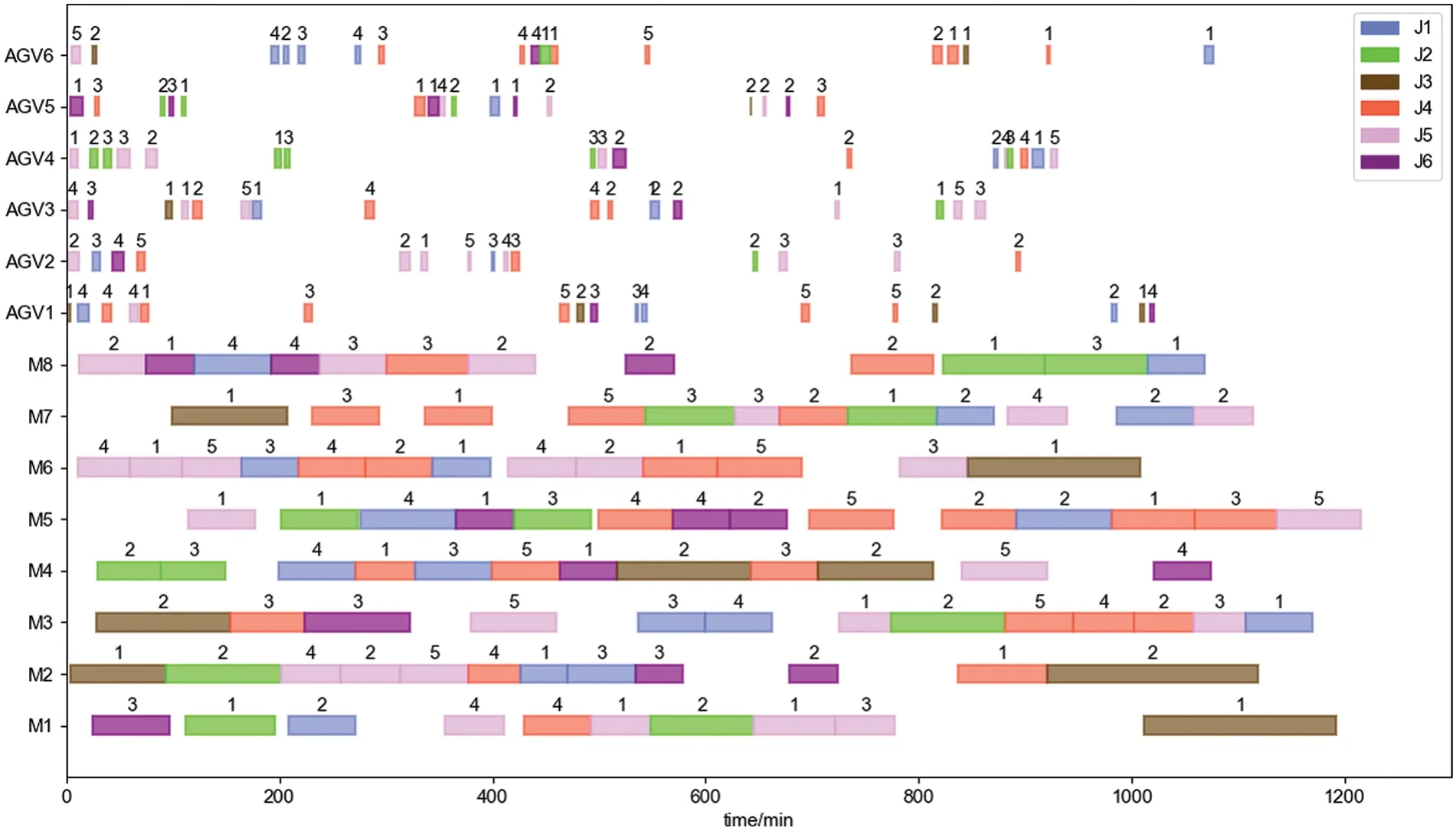
Figure 26:Scheduling scheme with 6 AGVs

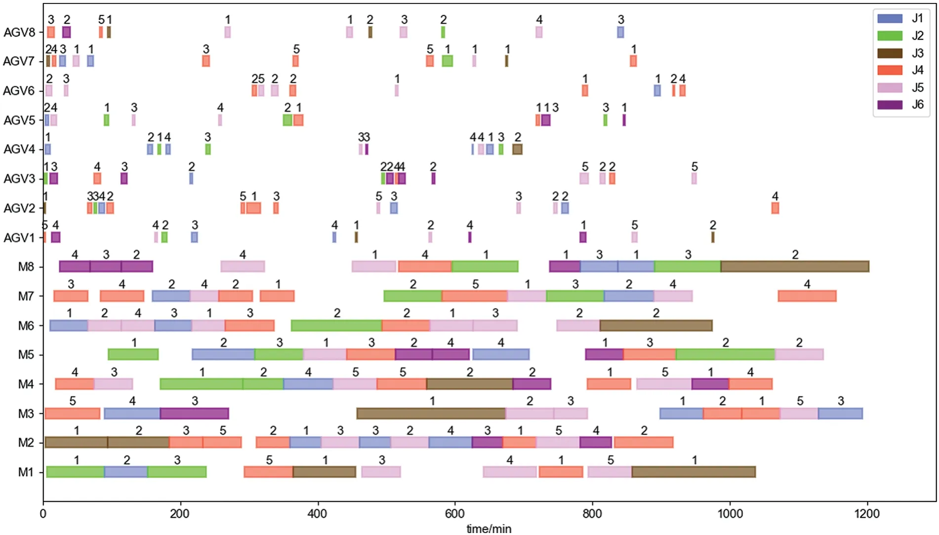
Figure 27:Scheduling scheme with 8 AGVs

5 Conclusion

To solve the dual-resource scheduling optimization problem of flexible job shops considering workpiece batching,this paper comprehensively considers workpiece batching,dual-resource scheduling and rescheduling problems.This paper establishes a mathematical model of dual-resource flexible job shop scheduling considering workpiece batching with the optimization objective of minimizing the maximum completion time and designs an improved two-layer optimization algorithm.Meanwhile,a random event-driven rescheduling method is designed for randomly occurring disturbance events in the workshop production process.

The case shows that:

1.The improved two-layer optimization algorithm is less likely to fall into local optimal solutions during the iteration process compared to the ordinary two-layer optimization algorithm.

2.The improved two-layer optimization algorithm can handle the disturbing events in the meter shop well and achieve a good rescheduling program.

3.The improved two-layer optimization algorithm can find the optimal number of AGVs in the actual operating environment.

The solving method proposed in this study combines with the actual production process,reduces the production cost of flexible operations to a certain extent and provides a new way of thinking for subsequent research.Meanwhile,it should be admitted that there are still some defects in the modeling process and the algorithm design process.In future research,we will increase the constraints to make it closer to the actual production,such as considering AGV power shortage,so that the disturbance events will be complete to better fit the actual situation.

Acknowledgement:Thank you to Nengjian Wang and Shuo Li for their technical and equipment support.

Funding Statement:The authors received no specific funding for this study.

Author Contributions:Study conception and design:Q.H.Liu,L.Z.Zhu;Program development:Z.J.Gao,L.Z.Zhu;Analysis and interpretation of results: J.Li;Draft manuscript preparation: L.Z.Zhu,J.L.Wang.All authors reviewed the results and approved the final version of the manuscript.

Availability of Data and Materials:The data in this article are all from computer simulation,and the data results refer to Tables 6 and 7 in the article.If you have any other questions,you can send an email to liuqinhui@hrbeu.edu.cn for communication and discussion.

Conflicts of Interest:The authors declare that they have no conflicts of interest to report regarding the present study.