Software Defect Prediction Method Based on Stable Learning

Xin Fan ,Jingen Mao ,Liangjue Lian ,Li Yu ,Wei Zheng and Yun Ge

1College of Aerospace Engineering,Nanjing University of Aeronautics and Astronautics,Nanjing,210012,China

2School of Software,Nanchang Hangkong University,Nanchang,330029,China

3Software Testing and Evaluation Center,Nanchang Hangkong University,Nanchang,330029,China

ABSTRACT The purpose of software defect prediction is to identify defect-prone code modules to assist software quality assurance teams with the appropriate allocation of resources and labor.In previous software defect prediction studies,transfer learning was effective in solving the problem of inconsistent project data distribution.However,target projects often lack sufficient data,which affects the performance of the transfer learning model.In addition,the presence of uncorrelated features between projects can decrease the prediction accuracy of the transfer learning model.To address these problems,this article propose a software defect prediction method based on stable learning(SDP-SL)that combines code visualization techniques and residual networks.This method first transforms code files into code images using code visualization techniques and then constructs a defect prediction model based on these code images.During the model training process,target project data are not required as prior knowledge.Following the principles of stable learning,this paper dynamically adjusted the weights of source project samples to eliminate dependencies between features,thereby capturing the“invariance mechanism”within the data.This approach explores the genuine relationship between code defect features and labels,thereby enhancing defect prediction performance.To evaluate the performance of SDP-SL,this article conducted comparative experiments on 10 open-source projects in the PROMISE dataset.The experimental results demonstrated that in terms of the F-measure,the proposed SDP-SL method outperformed other within-project defect prediction methods by 2.11%–44.03%.In cross-project defect prediction,the SDP-SL method provided an improvement of 5.89%–25.46%in prediction performance compared to other cross-project defect prediction methods.Therefore,SDP-SL can effectively enhance within-and cross-project defect predictions.

KEYWORDS Software defect prediction;code visualization;stable learning;sample reweight;residual network

1 Introduction

Embracing the swift advancements in science and technology,the software industry has emerged as a pivotal force in various applications,evolving from its subsidiary role for computer hardware to a diverse array of closed or open systems prevalent in contemporary times.Software defect prediction techniques have become significant tools in detecting possible software defects rapidly and accurately,thereby reducing software development costs and promoting software quality.Within the sphere of software defect prediction,researchers have classified historical training data into two categories:within-project defect prediction (WPDP) and cross-project defect prediction (CPDP) [1],based on whether the defects originate from the same project.

In studies focused on defect prediction,researchers have utilized machine learning techniques to extract a variety of features from software source code,aiming at higher accuracy of defect prediction models[2–6].Some scholars have sought to integrate program semantics into defect prediction features by employing a deep belief network(DBN)[6].This approach allows for the extraction of semantic features from the abstract syntax tree (AST) of the source code.Besides,a convolutional neural network(CNN)[7]has been deployed to autonomously capture both semantic and structural features of the program.Transfer component analysis (TCA) [8] was employed to train data transfer while preserving the data attributes,thereby ensuring the alignment of the source data distribution with that of the target data.Furthermore,a long short-term memory(LSTM)[9]network was engineered to parse the program’s structural information and code inter-relationships.However,a key aspect prevalent in these studies is the need for third-party tools to transform the code into another form,which might result in the loss of information related to code.

As a result,some certain scholars have chosen to forego the utilization of dedicated tools for intermediate code representation generation.Instead,they have adopted a more direct approach to enhance comprehensive feature extraction.Chen et al.[10] introduced a methodology involving software visualization and a deep transfer learning approach for defect prediction(DTL-DP).DTLDP creates code images at a fundamental granularity level through visualization techniques,mitigating the information loss attributed to manual feature determination or abstract syntax tree (AST)transformations.Nonetheless,DTL-DP exhibits two limitations.

For one thing,DTL-DP utilizes the deep transfer approach to learn transferable features;however,this still requires target project data as a priori knowledge,whereas in practice,the data for target projects are often insufficient,and the method of solving for the differences in the distribution of the sample data through transfer learning may result in negative transfer in some projects.

For another,the DTL-DP method ignores the impact of uncorrelated features on prediction performance,as shown in Fig.1.In the example code and saliency map of Fig.1,the brightness of the saliency map indicates the extent to which the model pays attention to specific regions of the input image,that is,brighter regions play a more important role in prediction.As shown in the figure,the presence of uncorrelated features and false correlations between uncorrelated features cause DTL-DP to focus on the entire image,whereas the proposed model focuses mainly on the core where code defects exist.In real software defect prediction tasks,the erroneous correlation between irrelevant features and code defects is a major factor causing model performance degradation,which is hard to evade while concentrating on the entire image,as in previous approaches such as DTL-DP.

To tackle these challenges,this study introduces a stable learning-based software defect prediction(SDP-SL) model,aiming to enhance the performance of software defect prediction.In particular,the initial stage of SDP-SL involves transforming code into images using software visualization techniques.Subsequently,dependencies between features are eradicated through global sample reweighting,emphasizing features more pertinent to code defects for classification purposes.Ultimately,SDP-SL is employed to extract features associated with code defects for defect prediction.Experimental findings demonstrate that the SDP-SL method outlined in this study yields superior outcomes compared to existing methodologies.

Figure 1:Saliency maps produced by the DTL-DP and SDP-SL models

The primary contributions of this study are outlined as follows:

1.We design the SDP-SL method,incorporating a sample reweighting technique to eradicate dependencies between features,allowing the model to concentrate on features directly associated with code defects.

2.Experimental evaluations conducted on 10 open Java projects demonstrate the enhanced performance of the proposed approach compared to WPDP and CPDP methodologies.

The subsequent sections of this paper are structured as follows:In Section 2,a literature review has been conducted.Section 3 dissects the SDP-SL method,followed by the presentation of the SDP-SL experimental setup in Section 4.The performance of SDP-SL is illustrated in Section 5,while potential threats to its validity are deliberated in Section 6.Finally,Section 7 draws a conclusions and proposes several potential avenues for future research.

2 Related Work

Stable learning (SL) was proposed to address high-risk fields,such as autonomous driving and healthcare.The core idea of SL is to realize the statistical independence of each dimensional feature through sample reweighting so that the association (correlation) between the reweighted outcome variable and each dimensional feature becomes a real causal relationship[11].SL methods consistently display good performance when using non-smooth and agnostic test data to learn models.Many machine learning methods that assume test and training data distributions to be consistent,have performed effectively.However,in practice,this assumption is often difficult to fulfill because models tend to exploit subtle statistical relationships between features when making predictions on test data,which makes them prone to prediction errors.

Consequently,researchers have proposed various solutions.For example,Liu et al.[12] applied density ratios to reweigh the training data to make the distribution closer to that of the test data.However,estimating the density ratio requires a priori knowledge on the test data distribution.Hu et al.[13] enhanced the ability of their model to generalize previously unseen domains by extracting domain-invariant features from multiple source domains.As model prediction performance is affected by the correlation between features,numerous studies were conducted to eliminate the correlation between features during training.Takada et al.[14] achieved feature decorrelation by using a regularizer to select highly correlated features.However,these methods are limited to the linear framework.Zhang et al.[15]innovatively proposed StableNet,which can process complex data types,such as images or videos.Nevertheless,SL method have not yet found application in defect prediction.In this investigation,we introduce an innovative stable learning-based mechanism that addresses feature decorrelation in defect prediction through sample reweighting.

Software defect prediction (SDP) stands as a prominent area of study in the field of software engineering.The majority of research efforts are directed toward extracting multifaceted features from software source code.These features’intrinsic interconnections are typically harnessed to train machine learning-based classifiers,predicting the defectiveness of code files.Among these,static and changing features have been widely confirmed by scholars.Static features include Halstead’s feature,which assesses code complexity based on the number of operators and operands[16];McCabe’s feature,which measures the complexity of the control flow in code based on code dependencies[17];and CK’s feature,which assesses the complexity of object-oriented software based on object-oriented concepts[18].None of the above features can be separated from the term“code complexity,”which is determined by a presupposition of applying the above features to construct software defect prediction models.That is,the more complex the structure of the source program code,the greater is the likelihood of the presence of defects.In many studies,changes in features have been proven to be effective in predicting software quality,including the number of code modifications [19],historical commit information[20],and code change records[21].Nevertheless,the static and change features utilized in the studies mentioned above are prone to subjective human interpretation and lack the inherent structural or semantic information contained by the code.

Therefore,some scholars have proposed constructing defect prediction models using the structural and semantic features contained in the code.Wang et al.[6] used a DBN to learn semantic features from token vectors extracted using an AST.Li et al.[7]used a CNN to generate features from the AST representation of the source code and attempted to combine it with some of the static features to further improve the model accuracy.In addition,because the WPDP is limited in practice,it is usually difficult for new projects to obtain sufficient training data;therefore,some scholars have turned to constructing predictive models by deploying other projects,among which transfer learning has gained attention.Nam et al.[22]proposed the TCA+method to enhance the performance of defect prediction models by mapping the source and target projects onto a potential feature space.Chen et al.[23] proposed double transfer boosting(DTB)to eliminate some of the instances by using Bayesian-based transfer enhancement.

Utilizing AST for code transition representation is flawed because the AST method is affected by granularity and fails to completely represent the information of the code.Therefore,Chen et al.[10]used code visualization technology [24] to convert code files into images,and then deep learning technology was adopted to extract features from the images,promoting the model’s performance.Table 1 summarizes and compares the existing methods.

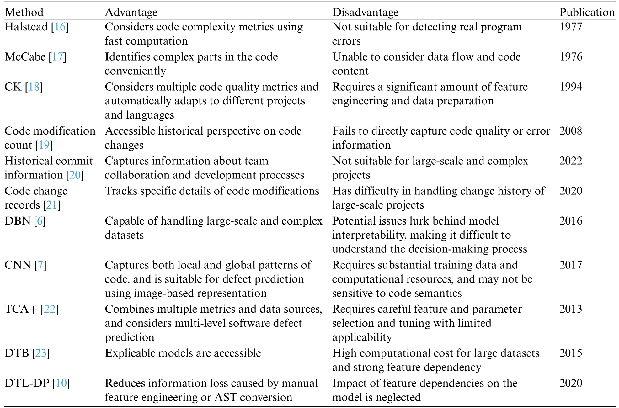
Table 1: Summary of existing methods

Inspired by the techniques mentioned above,this paper proposes the use of stable learning techniques based on code visualization,to eliminate the dependencies between features by training the weights of source project samples and navigating the focus of the model to real connections between code defect features and labels,thereby facilitating defect prediction performance.

3 Approach

The general framework of the SDP-SL methodology is delineated in Fig.2,comprising three stages: (1) generating code file visualization images,(2) constructing SDP-SL models,and (3) performing defect prediction.Initially,code files for each project are transformed into images using code visualization techniques.Subsequently,a defect prediction model is developed based on the RestNet18 network structure,incorporating a sample reweighting module to formulate the final SDP-SL model.In the final step,the test data are inputted into the trained SDP-SL model for defect prediction.Detailed explanations of each step follow in the subsequent sections.

3.1 Code File Visualization

In this step,we convert all code files of the source project into corresponding RGB images,as shown in Fig.3.First,the source code features in each code file are converted into corresponding ASCII decimal values.For example,the symbol‘+’is converted to“43”and the letter“M”is converted to“77”,following which,all features in the code file are combined into an integer vector,and all three values in the vector are grouped together.In order to convert the integer vector into pixels with color information,we specify these three values as the values of the color channels R,G,and B.For example,the word“and”which is common in code,can be converted to(97,110,100),whereby a lime green pixel is obtained by filling the RGB color channel with these three values in sequence;The word “static”can be converted to(115,116,97)and(116,105,99),to obtain two consecutive dark gray-green pixels and sepia pixels.This process is then repeated.

Figure 2:Framework of SDP-SL

Figure 3:Code file to code image

After the above operation,the pixel vector that is obtained has length one-third of the original(because every group of three features represents one pixel).The size of an image is affected by its width,and an image with an inappropriate width affects the predictive performance of subsequent models.According to the literature[25],it is more appropriate to determine the image width based on the size of the original code file.Therefore,the image width corresponding to files with a size of less than 10 KB was set to 32;for files between 10–30 KB,it was set to 64;for files between 30–60 KB it was set to 128;for files between 60–100 KB it was set to 256;for files between 100–200 KB,it was set to 384;and for files larger than 200 KB the width was set to 512.The specific code file visualization process is presented in Algorithm 1:

3.2 Modeling SDP-SL

The structure of SDP-SL is shown in Fig.4.The code image pass through a series of convolutional and pooling layers for feature extraction in a ResNet18 network and then through a global average pooling layer for the final features.These features are then fed into the global sample reweighting module(GSRM).Specifically,the first half of the GSRM performs sample weighting using random Fourier features(RFF),and the second half learns global sample weights.The weights learned by the GSRM module are combined with the predicted loss to obtain the final loss,to complete the training of the model.Next,ResNet18 and GSRM in SDP-SL are described in detail.

Figure 4:Network structure of SDP-SL

1) ResNet18 in SDP-SL: ResNet18 is a deep convolutional neural network,and unlike the traditional network structure,it introduces a residual structure to solve the degradation problem caused by an excessive number of network layers,thereby avoiding information loss during feature extraction.The structure of the ResNet18 used in this study was as follows:

Input Layer:The input image size was 224×224×3,that is,224 pixels in height,224 pixels in width,and three channels(RGB image).

Layer 1:The convolutional layer had three input channels and 64 output channels with convolutional kernel size of 7×7,stride of 2,and padding of 3.Batch normalization and ReLU activation were performed in a follow-up step.

Layer 2:This is a maximum pooling layer with a pooling kernel size of 3×3,a step size of 2,and padding of 1.The function of this layer is to downsample the spatial dimension of the feature map and reduce the size of the feature map to 1/4 of the original size.

Layer 3: Four basic convolutional blocks were used.Each basic convolutional block consisted of two 3×3 convolutional layers and a skip connection.The number of input and output channels was 64 each.The size of the convolutional kernel was 3×3 with a step size of 1 and a padding of 1.Each convolutional layer was subjected to batch normalization and ReLU activation.In the first basic convolutional block,input feature maps were added before the final ReLU activation function via skip connections to preserve feature information.In the other basic convolutional blocks,the number of input and output channels was kept constant.

Layer 4:Four basic convolutional blocks were used.Each basic convolutional block had 64 input channels and 128 output channels.The other configurations were the same as those of the third layer.

Layer 5:Four basic convolutional blocks were used.Each basic convolutional block had 128 input channels and 256 output channels.The other configurations were the same as those of the third layer.

Layer 6:Four basic convolutional blocks were used.Each basic convolutional block had 256 input channels and 512 output channels.The other configurations were the same as those of the third layer.

Global average pooling layer:This layer was used to reduce the spatial dimension of the feature map to 1×1 while preserving the channel dimension,with a final output of 1×1×512.

2) Global sample reweighting module in SDP-SL: This study introduced GSRM,which significantly reduces storage usage and computational cost by saving and reloading the global correlation mechanism,making global decorrelation via sample reweighting applicable to deep models.The GSRM includes a sample-reweighting module and a module for learning the global sample weights.

(a)Sample reweighting module:In previous studies,the Hilbert-Schmidt independence criterion(HSIC) was often utilized to supervise feature decorrelation [26].However,this is not applicable to deep model training because of the high computational cost.In fact,the Hilbert-Schmidt paradigm in Euclidean space corresponds to the Frobenius paradigm[27],and the independence test can also be based on the Frobenius paradigm.Therefore,feature dependency within the representation space was eliminated through sample weighting,and independence was assessed utilizing RFF.This is specified as follows:

First assume that the partial covariance matrix is:

wherenAandnBare sampled fromHRFF,which denotes the function space of random Fourier features as follows:

whereuandvdenote the RFF mapping functions included in Eq.(2).To minimize the correlation between features,w is optimized as follows:

The sample weights w,representation function f,and prediction function g can be iteratively optimized during the training process to obtain the best results.

whereZ(t+1)=f (t+1)(X),L(·,·)denotes the cross-entropy loss function,and t denotes the timestamp.The initial weights of all samples were set to 1.

(b)Learning global sample weights:In deep learning tasks,the learning of global sample weights is difficult to achieve because of the huge storage and computational costs required,and the samples in each batch are usually not complete during the optimization process.Therefore,we save the data from the training process and feed this data back into the model before the next training session,thereby optimizing sample weights.Specifically,the first step is to optimize feature generation for sample weights in each batch and merge all features based on sample crosstabs,as follows:

Znewdenotes the features used to optimize the weights of new samples;wnewdenotes the weights of new samples;Zcdenotes the features of the samples in the current batch;wcrefers to the weights of the samples in the current batch;andZG1,ZG2,...,ZGk,wG1,wG2,...,wGkrepresent the global features and weights,respectively,updated at the end of the training of each batch.We keptwGifixed at the beginning of training in each batch,which makes onlywclearnable.Therefore,as soon as a training iteration of the model concludes is completed,we integrate local information(Zc,wc)and global information(ZGi,wGi),as follows:

whereαirepresents the smoothing parameter,which serves to balance the long-term memory and short-term memory in the global information.Finally(ZGi,wGi)was updated to

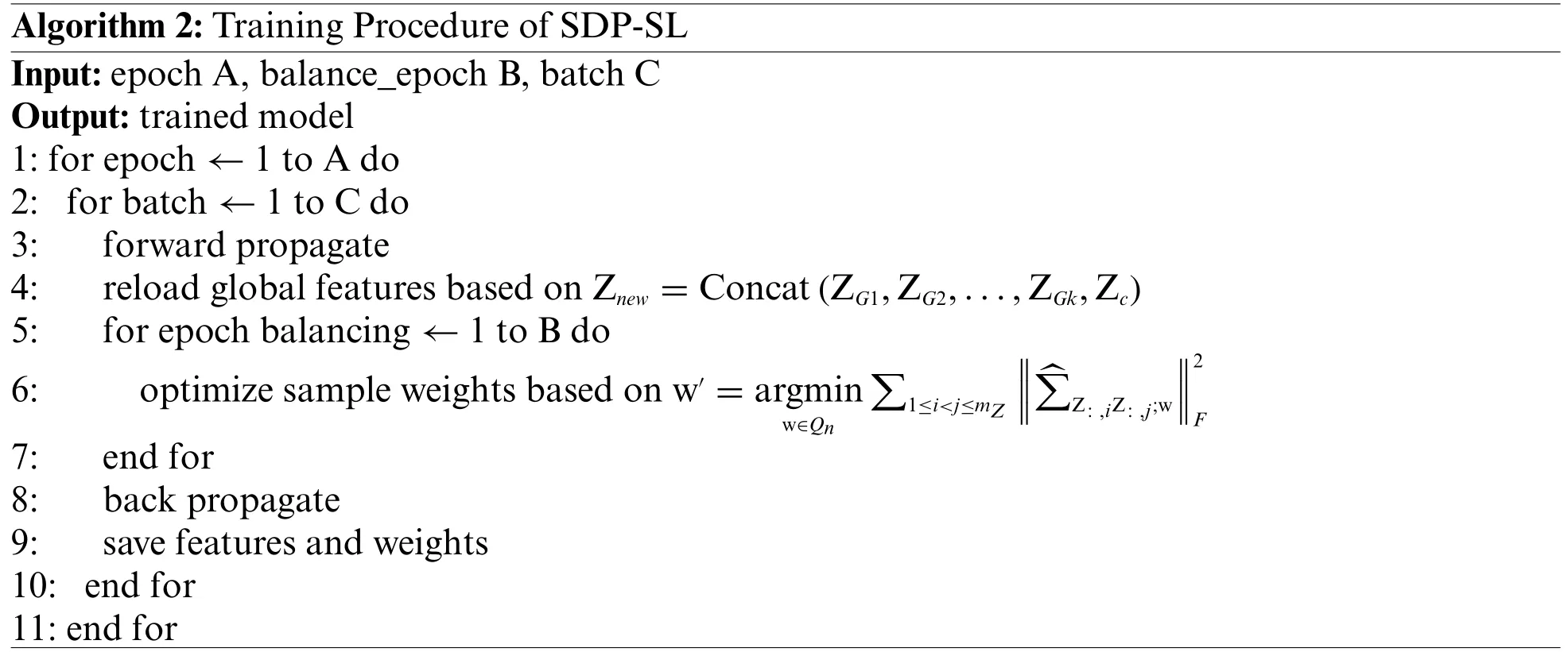
The training procedure for our SDP-SL is shown in Algorithm 2:

3.3 Execute Defect Prediction Tasks

When training the SDP-SL model,the visualization images generated by the source project are input into the model,whereby the model iteratively optimizes the sample weights and model parameters during the training process.In the prediction phase,the model can directly predict the presence of code defects in input projects without any other calculation.

4 Experiments

Experiments were conducted to evaluate the performance of SDP-SL,including WPDP and CPDP defect prediction,and the results were compared with several existing deep-learning-based defect prediction methods.The average results were reported after running each experiment ten times.Next,we provide a detailed introduction to the dataset,baseline methodology,statistical tests,and evaluation metrics.

4.1 Dataset Description

For a convenient and smooth comparison of our work and that of other scholars,we borrowed a dataset from the literature [10],which is publicly available in the PROMISE3 database.Different versions of each of the 10 Java projects were obtained from GitHub,thereby recording the project name,version number,and defect labels for each of the code files in these projects.Efforts were also made to count the total number of files available,average file size,and average defect rate for each project.Detailed information about the 10 projects is provided in Table 2.In the WPDP experiments,sequential versions of each project,as outlined in Table 1,were utilized for defect prediction.Specifically,the older versions were chosen for model training,while the newer versions serving as the target project for testing(e.g.,the lucene-2.0 project was employed as the training set,and the lucene-2.2 project was designated as the test set).In the CPDP experiments,one version was randomly selected from each project as the target project,and two projects distinct from the target project were chosen as the source projects for defect prediction.

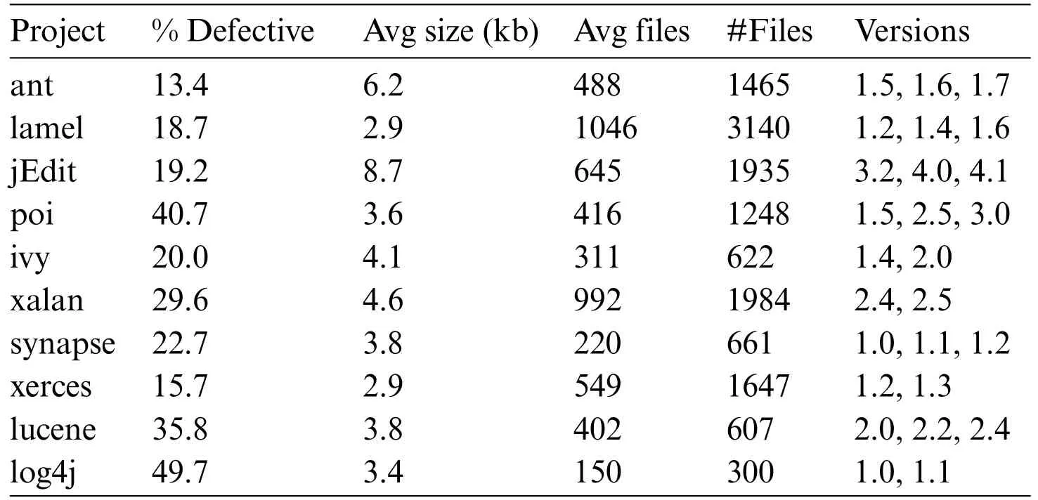
Table 2: Dataset details

4.2 Baseline Methods

To comprehensively evaluate the prediction performance of the SDP-SL model for WPDP and CPDP software defect prediction,we compared it with various benchmark methods,as shown in Table 3.The details of this process are described below:

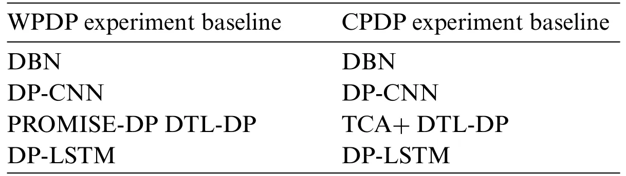
Table 3: Baseline method selection

• DBN This is a deep learning model that can improve defect prediction performance by learning advanced features,such as semantic features,in software projects.

• DP-CNN:Deep pyramid CNN is a CNN-based software defect prediction method that focuses on learning feature representations from the AST structure of the source code.DP-CNN can effectively capture pattern and structure information in the code,thereby enhancing the accuracy of defect prediction.

• DP-LSTM:Differential privacy-inspired LSTM is a software defect prediction method based on LSTM,which is a recurrent neural network.In software defect prediction,DP-LSTM utilizes the LSTM network to construct the evolutionary history and change patterns of the code,to predict potential defects.

• DTL-DP:This is the latest defect prediction model,which employs the approach of converting code into images combined with attention mechanisms,effectively enhancing the model’s performance.

• PROMISE-DP:This is a method for defect prediction that utilizes static features,eliminating the need for source code as training data.It possesses a relatively straightforward structure.

In CPDP experiments,we used the TCA+method instead of PROMISE-DP for cross-project defect prediction because PROMISE-DP cannot be deployed directly.

• TCA+: This technique represents an advanced method for data transfer,preserving crucial data attributes while aligning the distributions of both source and target data.It utilizes TCA integrated with sophisticated algorithms,enabling seamless knowledge transfer across domains.

For a fair comparison,the same computer was used to conduct experiments and report the average results.The baseline method is implemented exactly as delineated in the relevant paper.

4.3 Statistical Test

To perform a multidimensional comparison between SDP-SL and other methods,we utilized the Scott-Knott effect size difference (ESD) test method.This technique employs a hierarchical clustering algorithm to group means and evaluates the statistical significance of differences between these clusters.The specific procedure is outlined as follows:

1)Finding the optimal grouping:First,the division that maximizes the mean value of component measurements is determined using hierarchical clustering.This step facilitates the grouping of samples with similar measurements to better compare their performances.

2)Grouping or merging:After obtaining the optimal grouping,certain combinations are merged into one group or a group is split into two groups based on the marked differences between the samples.The purpose of this step is to identify prominent differences between the groups to determine which models have a significant advantage in performance.

4.4 Evaluation Metric

For a comprehensive assessment of model performance and to ensure that the model is well balanced in positive and negative samples,we adopted the F-measure metric which combines two metrics,precision and recall,as the evaluation index of the model.The performance of the classification model cannot be evaluated without the confusion matrix,which records the four possible outcomes of the model’s classification of samples,as shown in Table 4.

Table 4: Confusion matrix

Specifically,if the model correctly predicts a flawless document as a positive example,it is called a TP;if the model incorrectly predicts a defective document as a positive example,it is a FP;if the model correctly predicts a defective document as a negative example,it is a TN;and if the model incorrectly predicts a flawless document as a negative example,it is a FN.The precision (P),recall(R),and F-measure are defined as follows:

5 Results

5.1 RQ1:How Does SDP-SL Compare to the Other Five Baseline Methods in WPDP?

This study compared SDP-SL with five baseline methods,including the PROMISE-DP method,which is based on traditional features for defect prediction;DP-CNN,which is based on AST for extracting semantic structural features;and the newest DTL-DP method,which combines software visualization and self-attention mechanisms.Sixteen sets of WPDP experiments were carried out utilizing these five methodologies.In each experiment,the old versions of the project were chosen to train the model with source data,while the new versions serving as the target project for testing purposes.

Table 5 shows the experimental results for all the methods in the WPDP experiments.The highest F-measure values for the six methods are indicated in bold.Each of the six methods was run 10 times on 16 sets of data to avoid random results.In the table,the average F-measure of SDP-SL is 0.628,and the average F-measures of DTL-DP,PROMISE-DP,DP-LSTM,DP-CNN,and DBN are 0.615,0.498,0.500,0.550,and 0.436,respectively,which is an improvement of 2.11%,26.10%,25.6%,12.42%,and 44.03%,respectively.The results show that,compared with DBN,DP-CNN,DP-LSTM,PROMISE-DP,and DTL-DP,the proposed method is highly competitive in improving within-project defect prediction.

Table 5: F-measure of the six methods in the WPDP experiments

In the second-to-last row of Table 5,W/T/L signifies the count of wins,draws,and losses when comparing SDP-SL results with those of the corresponding method in the current column.The most favorable outcome observed was 16 wins,0 draws,and 0 losses,while the least favorable outcome was 14 wins,0 draws,and 2 losses.Hence,the findings affirm the positive impact of the SDP-SL method on within-project defect prediction.

In the experiments,the Scott-Knott ESD test was applied to the prediction results of each method,and the results are shown in Fig.5.In the figure,the SDP-SL method not only has the highest average F-measure in the WPDP experiments but also a higher median value than all other methods.The results of the Scott-Knott ESD test demonstrate the superiority of the SDP-SL method for withinproject defect prediction,where it excels in terms of average F-measure and performance stability,displaying better prediction performance and reliability.

Overall,the results of the experimental and statistical validations show that the SDP-SL method is effective for WPDP and can improve the performance of WPDP tasks.

5.2 RQ2:How Does SDP-SL Compare to the Other Five Baseline Methods in CPDP?

As described in Section 4.2,TCA+was used to replace PROMISE-DP in the CPDP experiments.We conducted 22 sets of CPDP experiments,in which one version from each project was randomly selected as the target project,and the source project comprised two projects different from the target project.

Table 6 presents the experimental results for all methods in the CPDP experiment.The highest F-measure values for the six methods are indicated in bold.Each of the six methods was run 10 times on 22 sets of data to avoid random results.In the table,the average F-measure of SDP-SL is 0.611,and the average F-measures of DTL-DP,TCA+,DP-LSTM,DP-CNN,and DBN are 0.577,0.487,0.490,0.536,and 0.561,respectively,resulting in improvements of 5.89%,25.46%,25.46%,and 8.91%,respectively.The results show that the proposed method provides significant advantages over other baseline methods in terms of improving cross-project defect prediction.

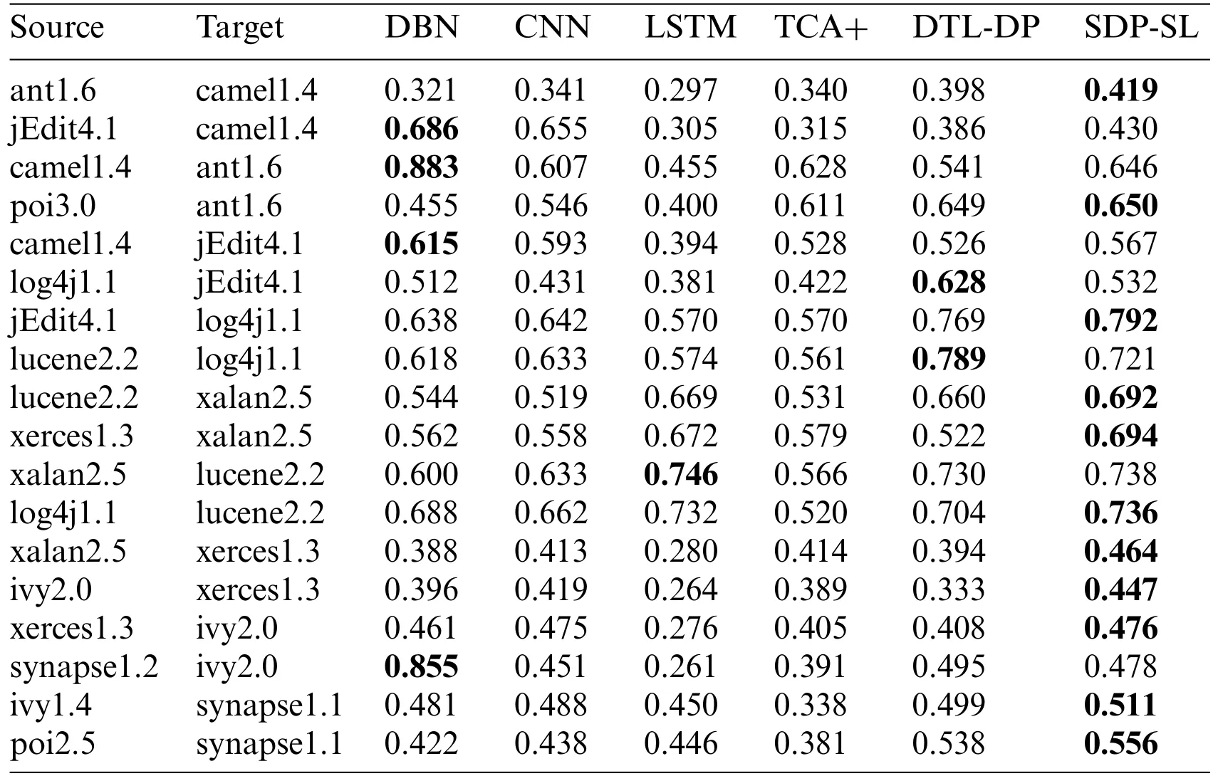
Table 6: F-measure of the six methods in the CPDP experiments

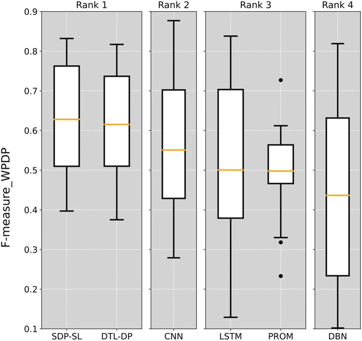
Figure 5:Scott-Knott ESD test on six different WPDP defect prediction methods

In CPDP,the comparison of victories,draws,and losses between the SDP-SL method and other approaches is evident from the penultimate row of Table 6.The most favorable outcome observed was 20 wins,0 draws,and 0 losses,while the least favorable outcome was 16 wins,0 draws,and 4 losses.Therefore,the results indicate that the SDP-SL method is highly effective in CPDP.

As described in Section 5.1,a Scott-Knott ESD test was conducted on the prediction results of each method,as shown in Fig.6.The average F-measure of the SDP-SL method is the highest throughout the CPDP experiments,and the median value of the SDP-SL method is also higher than that of all the other methods.The results of the Scott-Knott ESD test indicate the superiority of the SDP-SL method in cross-project defect prediction,with the prominent average F-measure and performance stability values,indicative of better prediction performance and reliability.

Figure 6:Scott-Knott ESD test on six different CPDP defect prediction methods

In summary,the experimental and statistical validation results demonstrate that the SDP-SL approach is effective for CPDP and can improve the performance of CPDP tasks.

5.3 RQ3:Why Does the Proposed SDP-SL Approach Work?

The experimental results in Sections 5.1 and 5.2 demonstrate that the SDP-SL method has better prediction performance than the various types of baseline methods in the software defect prediction task,for both within-and cross-project defect prediction.There are two possible reasons for this finding.

1) Through code visualization,SDP-SL attempts to extract structural semantic features from letters,which,compared with other extraction methods (e.g.,hand-counted and AST-generated features),provide more comprehensive information and avoid information loss.

2)The SDP-SL method considers the impact of correlations between features on model performance.This research added a sample reweighting module based on the idea of stable learning to the model,thereby decorrelating features by weighting the samples,to obtain feature information that is directly related to code defects for training.

5.4 Discussion

Regarding the choice of the base model,deep learning-based defect prediction models have several significant advantages over static and dynamic code analysis tools.First,deep learning models can learn patterns and features from large-scale source code,enabling them to detect more complex code defects,including those that may be difficult to identify using traditional code-analysis tools.In addition,deep learning models can continuously learn and improve their performance through training and iterations,allowing them to adapt to new code defect patterns and project requirements.To address the issue of vanishing gradients that may arise during the training process,ResNet was selected as the base model.The residual connections in ResNet allow information to be directly propagated between layers,effectively mitigating the problem of vanishing gradients.ResNet has been widely applied in deep learning frameworks,demonstrating excellent performance,particularly in various image-related tasks.By transforming source code files into code images,the goal is to conveniently leverage image-based models,such as ResNet,for defect prediction while preserving program details to the maximum extent possible.

6 Threats to Validity

Threats to internal validity: To prove the validity of the SDP-SL method,we compared it with several baseline methods.Among these baseline methods,if the source code was available in the original paper,we utilized that code to implement the corresponding baseline method.For some of the methods with no source code available in the original paper(e.g.,DP–CNN),we strictly followed the details in the original paper,to maintain consistency as much as possible.

Threats to external validity: Datasets from 10 different projects were used in the experiments,covering 16 sets of within-project defect prediction and 22 sets of cross-project defect prediction tasks.We deliberately selected diverse datasets of varying sizes and defect rates,to ensure reliability of the experimental results.Nevertheless,while this method exhibits sound performance in Java projects,there is no assurance that our approach will yield similar enhancements when applied to distinct programming languages.

Threats to construct validity: The F-measure,which has been widely used in previous studies,was chosen as the evaluation metric to assess the validity of defect prediction.The F-measure is a comprehensive metric that balances accuracy and recall and is widely applied in the performance evaluation of defect prediction.Although we believe that the F-measure is a reliable performance metric,different conclusions may be reached with other performance metrics.

7 Conclusions and Future Work

This study introduces a defect prediction method called SDP-SL,which combines stable learning with code visualization.By converting code into images and utilizing a ResNet18 network with a sample reweighting module,SDP-SL enhances features by giving different weights to samples.It enables the model to identify crucial defect-related features,improving defect prediction performance.Our experimental results validate the superiority of SDP-SL over other baseline methods.

However,SDP-SL has some limitations.During the conversion of code files into code images,there may be some loss of information,which can influence the predictive performance of the model.Therefore,in future research,we will explore methods to preserve source code information more effectively while transforming code files into code images.Additionally,manual parameter settings may have impacted the model’s predictive performance.Therefore,future research will incorporate parameter optimization techniques to automatically fine-tune the model parameters and strive for even better performance.

Acknowledgement:The authors would like to express appreciation to the National Natural Science Foundation of China(Grant No.61867004)and the National Natural Science Foundation of China Youth Fund(Grant No.41801288)for their financial support.We would like to thank Editage(www.editage.cn)for English language editing.

Funding Statement:This research was supported by the National Natural Science Foundation of China(Grant No.61867004) and the Youth Fund of the National Natural Science Foundation of China(Grant No.41801288).

Author Contributions:The authors confirm contribution to the paper as follows: study conception and design: X.Fan,J.Mao,L.Lian,L.Yu,W.Zheng;data collection: X.Fan,J.Mao,L.Lian,L.Yu;analysis and interpretation of results:X.Fan,J.Mao,L.Lian,L.Yu,W.Zheng;draft manuscript preparation: X.Fan,J.Mao,L.Lian,L.Yu,W.Zheng,Y.Ge.All authors reviewed the results and approved the final version of the manuscript.

Availability of Data and Materials:The data that support the findings of this study are openly at:https://github.com/maojingen/SDP-SL.

Conflicts of Interest:The authors declare that they have no conflicts of interest to report regarding the present study.