A Composite Transformer-Based Multi-Stage Defect Detection Architecture for Sewer Pipes

Zifeng Yu ,Xianfeng Li,⋆ ,Lianpeng Sun ,Jinjun Zhu and Jianxin Lin

1School of Computer Science and Engineering,Macau University of Science and Technology,Macau,999078,China

2School of Environmental Science and Engineering,Sun Yat-sen University,Guangzhou,510275,China

3Guangdong AIKE Environmental Science and Technology Co.,Ltd.,Zhongshan,528400,China

ABSTRACT Urban sewer pipes are a vital infrastructure in modern cities,and their defects must be detected in time to prevent potential malfunctioning.In recent years,to relieve the manual efforts by human experts,models based on deep learning have been introduced to automatically identify potential defects.However,these models are insufficient in terms of dataset complexity,model versatility and performance.Our work addresses these issues with a multi-stage defect detection architecture using a composite backbone Swin Transformer.The model based on this architecture is trained using a more comprehensive dataset containing more classes of defects.By ablation studies on the modules of combined backbone Swin Transformer,multi-stage detector,test-time data augmentation and model fusion,it is revealed that they all contribute to the improvement of detection accuracy from different aspects.The model incorporating all these modules achieves the mean Average Precision (mAP) of 78.6% at an Intersection over Union(IoU)threshold of 0.5.This represents an improvement of 14.1%over the ResNet50 Faster Region-based Convolutional Neural Network (R-CNN) model and a 6.7% improvement over You Only Look Once version 6(YOLOv6)-large,the highest in the YOLO methods.In addition,for other defect detection models for sewer pipes,although direct comparison with them is infeasible due to the unavailability of their private datasets,our results are obtained from a more comprehensive dataset and have superior generalization capabilities.

KEYWORDS Sewer pipe;defect detection;deep learning;model optimization;composite transformer

1 Introduction

Sewerage systems are a fundamental component of urban infrastructure for treating and removing both sewage and rainwater.However,sewer pipes are long-term infrastructure and susceptible to various defects.If these defects are not repaired timely,they can cause further deterioration and require more complex repair or replacement work [1].Unhealthy sewers can also cause serious problems such as sewer overflows (SSOs) and urban pavement collapse,leading to environmental damage,property damage,and injuries[2,3].Sewer defect detection can help find hidden or covered manholes or unknown pipe segments in the drainage system,find and identify the sources and connections of illegal sewage discharge,investigate the causes of pipe blockage and poor drainage,and detect pipe damage,mismatch,deposition,sewage leakage and pollution.Automatic sewer defect detection can effectively prevent urban disasters such as water logging,pollution,disease,etc.,and improve the ecological environment and living quality of the city.

Currently,Closed Circuit Television (CCTV) technology is widely used to inspect underground sewage pipes [4].The Operator controls the crawler’s speed and direction in the pipe using a master controller,transmitting inspection videos to the main controller monitor via a cable.In real-time,operators can monitor the video,identify pipeline defects,and capture defect images.The video frames can also be stored and analyzed later.However,this defect identification demands specialized skills and heavy labor.Automatic defect identification of sewer pipes is highly desired and has become an intensively researched topic in recent years.

In the past decade,deep learning has made significant progress in image recognition,especially with the success of deep learning-based object detection,providing researchers with novel methods and opportunities for automated sewer defect detection.For instance,researchers from Canada and Massachusetts Institute of Technology [5] introduced an algorithm based on convolutional neural networks (CNN) for detecting cracks on building surfaces,with an accuracy of 98%.However,this algorithm is specialized for a single defect class,such as cracks.Hassan et al.[6]took a unique approach by directly analyzing sewer CCTV video,extracting characteristic frames,and incorporating a preprocessing step to eliminate textual captions from the video frames.Yin et al.[7]used the improved one-stage You Only Look Once version 3 (YOLOv3) as the base model to detect six defect classes,achieving a final mean Average Precision(mAP)of 85.37%.Similarly,Tan et al.[8]also used YOLOv3 as the basic model and further refined it with YOLOv4 and YOLOv5 methods,resulting in a mAP of 92%for four sewer defect classes.Cheng et al.[2]proposed a deep learning-based object detection model based on an improved two-stage Faster Region-based Convolutional Neural Network(R-CNN)algorithm.This model integrates a defect Region Proposal Network(RPN)with convolutional feature maps to achieve classification and localization of four defect classes,with a mAP of 83%.Dang et al.[9]used a modified ResNet50 detection transformer model for sewer defect object detection,attaining an mAP of 60.3%following the Common objects in context evaluation criteria.

The mentioned sewer defect detection solutions have shown improved performance.Nevertheless,research in this area is still in its early stages.The range of relevant datasets used by the algorithms is limited and the effectiveness of the techniques has not yet been fully explored.Thus,there is a clear need for further research in this field.

In recent years,the transformer has shown superior performance than CNN in a variety of image challenges[10–13].On the other hand,object detection architectures are mainly classified into anchorfree models[14],single-stage models[15],two-stage models[2],and multi-stage models[16].It has been shown that two-stage is more likely to achieve superior precision than single-stage when there is more training data on sewer defects [17].Inspired by previous work,a novel multi-stage object detection model based on a composite backbone Swin Transformer is designed for detecting sewer defects.We have also investigated the different factors that affect the performance of the model.It has also been compared with other high-performance sewer defect detection architectures.The main contributions of this study are as follows:

1.A dataset with 6756 sewer images,containing 9 classes of defects and 1 normal class has been collected.Fig.1 shows examples of these defects.

2.A multi-stage defect detection architecture using a composite backbone Swin Transformer for urban sewer pipes is proposed.This architecture can distinguish between normal and defective classes,as well as perform object detection for nine different classes of defects.

3.We have performed ablation experiments on the composite backbone,multi-stage detector,testtime data augmentation and model fusion methods to test the effectiveness of these modules in sewer defect detection.

4.The model achieves significant performance improvements over existing deep models.The mAP of our model achieves 78.6%at an Intersection over Union(IoU)threshold of 0.5(mAP@0.5).Our model demonstrates a 14.1% improvement compared to the ResNet50 Faster R-CNN and a 6.7%improvement compared to YOLOv6-large,which is the highest among the YOLO methods.

Figure 1:Nine classes of defects(a–i)in urban sewer pipes.(a)PL:Cracking;(b)AJ:Concealed joint;(c)CK:Mismatch;(d)TJ:Disjointed;(e)BX:Deformation;(f)SG:Root;(g)CJ:Deposition;(h)ZW:Barrier;(i)CR:Foreign body penetration

2 Methodology

Our composite sewer defect detection model consists of five parts,as illustrated in Fig.2.The first part performs data augmentation,which addresses the imbalanced distribution of defect classes,lighting,and low image qualities.The second part is the assisting backbone,which provides more feature information and regularization for the lead backbone.The third part is the lead backbone,which extracts image features for different defects and fusion the features of the assisting backbone.The second and the third parts form the composite backbone.The fourth part is the neck,which further fusion features from different levels of the lead backbone.The final part is the detection head,which predicts defects at various locations based on the features obtained from previous parts.The components designed for these parts are described below.

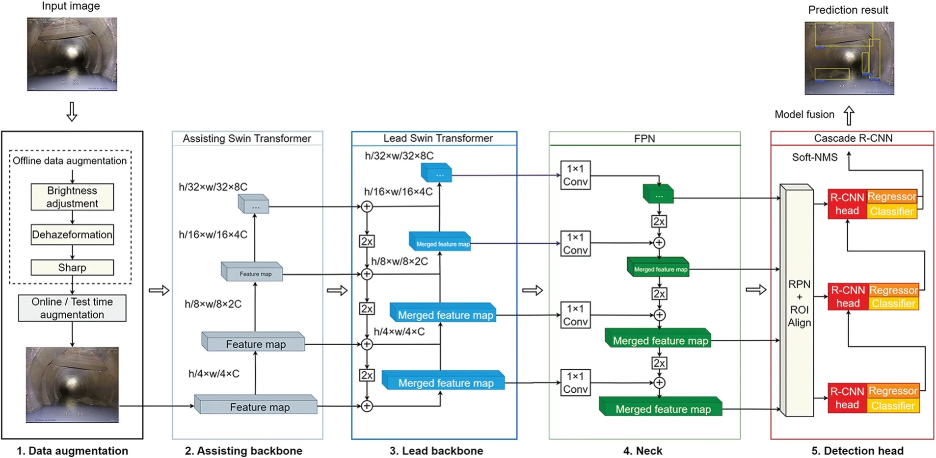
Figure 2:The architecture and flow of the multi-stage model

2.1 Data Augmentation

The poor conditions in sewer pipelines often result in low-quality images,such as bad illumination,and blurry,hazy,or noisy pixels.These problems pose more difficulties for feature extraction than other domains of object detection[18].Furthermore,sewer defects are quite imbalanced,with some types of defects much rarer than other types.Data augmentation is proposed to address this issue.It is divided into two approaches:offline and online data augmentation.The former is used to improve the image quality.Denoising and brightness adjustment,DehazeFormer[19]and Sharpen augmentation are applied to all the images in the dataset.The latter is used to improve the generalization ability of the model by introducing randomness in the training stage.Random flip and resize,Random color jitter and Gaussian noise are applied in this architecture.Fig.3 shows the effects of offline and online data augmentation.Where the online data augmentation is applied after offline data augmentation.

In addition,test-time data augmentation (TTA) is used to fuse the results of different data augmentations for each image during the test stage.As shown in Fig.4,the original image is resized and horizontally flipped.Unlike data augmentation during training,TTA averages the results of different image sizes and horizontal flips.It improves the model performance by incorporating multiple predictions for each image,resulting in more accurate and robust defect detection.

Figure 3:Effects of offline and online data augmentation

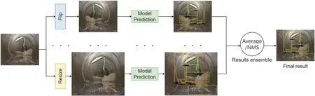
Figure 4:Schematic diagram of the TTA algorithm for object detection

2.2 Swin Transformer

The Swin Transformer (large version) is used as the foundational infrastructure for feature extraction in our architecture.Fig.5 illustrates the processing flow,where the input to the Swin Transformer is an RGB image(H×W×3)post-data augmentation.

Patch Partitioning is a method to divide an image into non-overlapping patches of equal size.Each patch is treated as a token for the Transformer.Specifically,our model employs the number of H/4× W/4 patches,each patch having dimensions of 4 × 4 × 3.This operation transforms the original image into a H/4×W/4×48 tensor.Linear Embedding is employed to map the feature dimensions of each patch.The dimensions of the image will transform into H/4×W/4×C,which facilitates the subsequent Transformer operations.

The feature extraction part of the Swin Transformer consists of four stages.Each of these stages is composed of a Patch Merging layer and Swin Transformer blocks.Patch merging is a method to merge adjacent patches into larger ones using linear transformation.It reduces the number of tokens and increases the receptive field of each token,similar to the pooling layer in CNN.It is the process of merging four adjacent patches into a new patch,simultaneously reducing the feature dimensions from 4C to 2C.

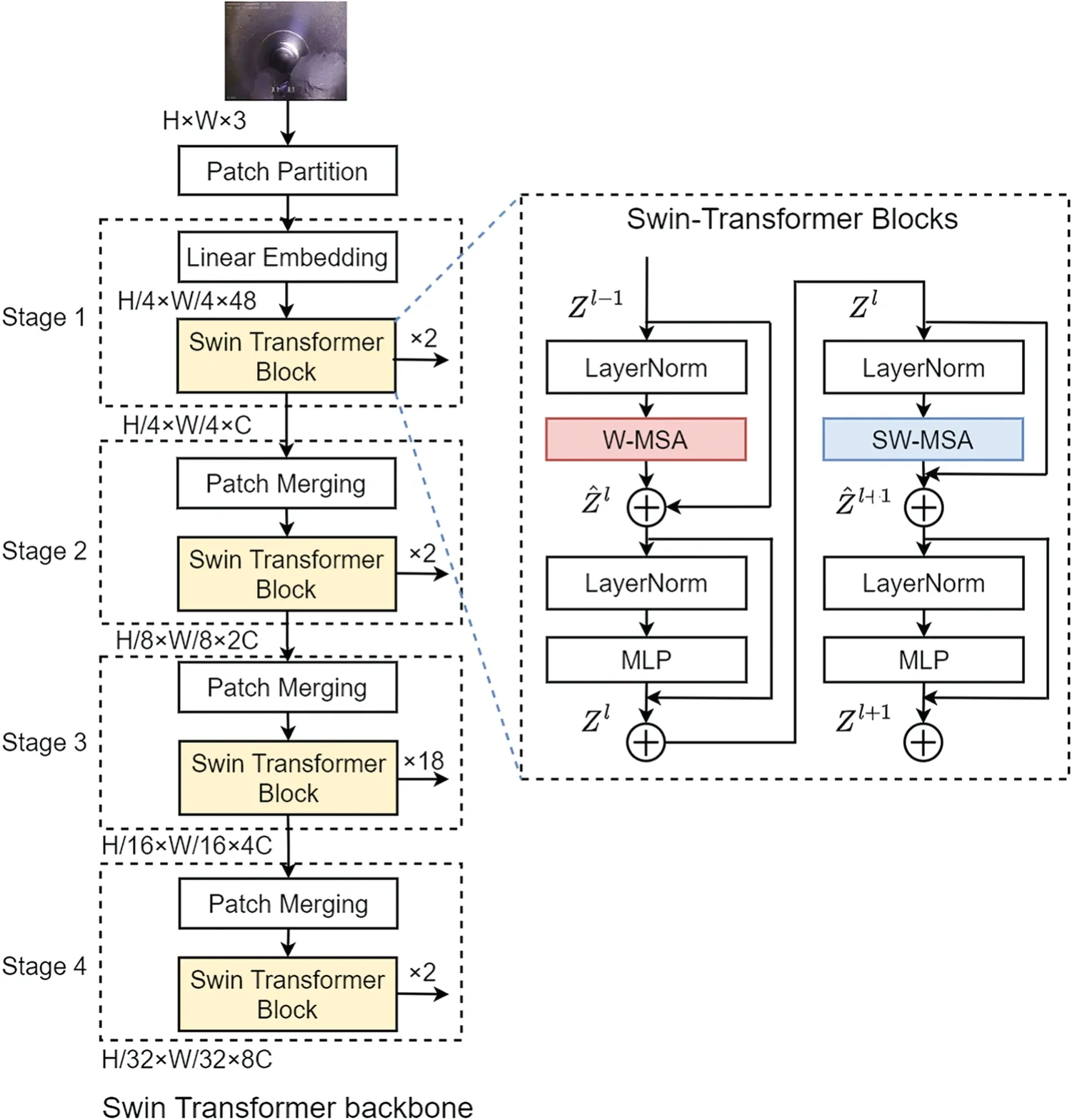
Figure 5:The architecture of CBSwin-Transformer

The Swin Transformer Block is the core module of the Swin Transformer network architecture.It is comprised of either the Window-based Multi-head Self Attention(W-MSA)module or the Shifted Window Multihead Self-Attention (SW-MSA) module,along with Layer Normalization and two layers of Multi-layer Perception Module(MLP).

W-MSA effectively partitions the input feature map into distinct,non-overlapping windows,conducting multi-head self-attention computations within each window.The computational formula for each window is as follows:whereQ,K,Vare thequery,key,andvaluematrices of dimensionM2×d,respectively,M2is the number of patches within a window,T denotes the transpose notation,dis thequeryorkeydimension,andBis the learnable relative position bias matrix with dimension ofM2×M2,utilized to enrich positional information.

While W-MSA can preserve local information interaction and reduce redundancy in the global self-attention computation,tokens can only interact with other tokens within the same window.This ignores the relationship between different regions in the image.To introduce cross-window connectivity while maintaining efficient computation in non-overlapping windows,W-MSA is employed alternatively with SW-MSA.SW-MSA is a method to compute the self-attention between tokens within shifted windows.The windows are shifted by half of their size across blocks so that each token can interact with the tokens from neighboring windows.The tokens in each window are processed by W-MSA,and then the output tokens are re-arranged to form the original grid.

The output of the Swin Transformer is a set of feature maps at different stages that will be used as input to the lead backbone or Feature Pyramid Network(FPN).

2.3 Composite Backbone and Neck

The single Swin Transformer provides global features of the image.To better identify defects that often occupy only part of an image,it is necessary to utilize local features,which have been extracted at different network layers of the backbone.Thus,an assisting Swin Transformer and FPN are designed to combine global features with local features for identifying objects of different sizes.

2.3.1 Composite Backbone Swin Transformer

The composite backbone Swin Transformer(CBSwin)consists of two identical Swin Transformers: the assisting Swin Transformer and the lead Swin Transformer.As shown in Fig.2,CBSwin integrates the high-level or same-level output features of the assisting Swin Transformer with the lowlevel features of the lead Swin Transformer to perform feature fusion.

At the model training stage,The assisting backbone has an auxiliary neck and an auxiliary detection head,which share parameters with the main neck and detection head.The auxiliary neck takes the output of the assisting backbone as input and produces multi-scale feature maps.The auxiliary detection head predicts the bounding boxes and class labels of the objects on the feature maps.The auxiliary branch will generate the assisting loss,denoted asLAssist.In summary,the total lossLis trained using the following loss function:

whereLleadis the loss of the main branch,andLAssistis the loss of the auxiliary branch.

The assisting loss introduces extra regularization during the training of the lead backbone,which prevents overfitting and improves the generalization performance of the model.

2.3.2 Feature Pyramid Network

FPN is used as a neck to fusion output features from different stages of the lead Swin Transformer.FPN consists of a bottom-up route,a top-down route,and a lateral connection,as illustrated in Fig.2.The FPN works as follows.First,the features extracted at each stage of the backbone are fed to a 1×1 convolution(Conv)in the FPN,which combines different feature maps at this level to form a set of feature maps consisting of 256 channels.These feature maps are then combined with features from higher levels with two times (2×) nearest interpolation upsampling.Meanwhile,these feature maps are also provided to the RPN network in the detection head for object region proposals.

2.4 Detection Head

The detection head makes predictions on sewer defects from the feature pyramid obtained by the neck part.Fig.2 shows the overall design of the detection head.It first produces a set of region proposals with the RPN,which are then pooled by the Region of Interest Align(ROIAlign)module.These region proposals are then selected and adjusted with regressions by the Cascade R-CNN predictor.

2.4.1 RPN and ROIAlign

RPN initially generates a series of anchors,representing potential defect regions,as shown in Fig.6a.Each anchor receives feature map information from the neck stage as input to the RPNHead.Subsequently,the classifier within the RPNHead predicts whether the anchor box area is the background or foreground.Simultaneously,the regressor adjusts the anchor box to better fit the ground truth box.

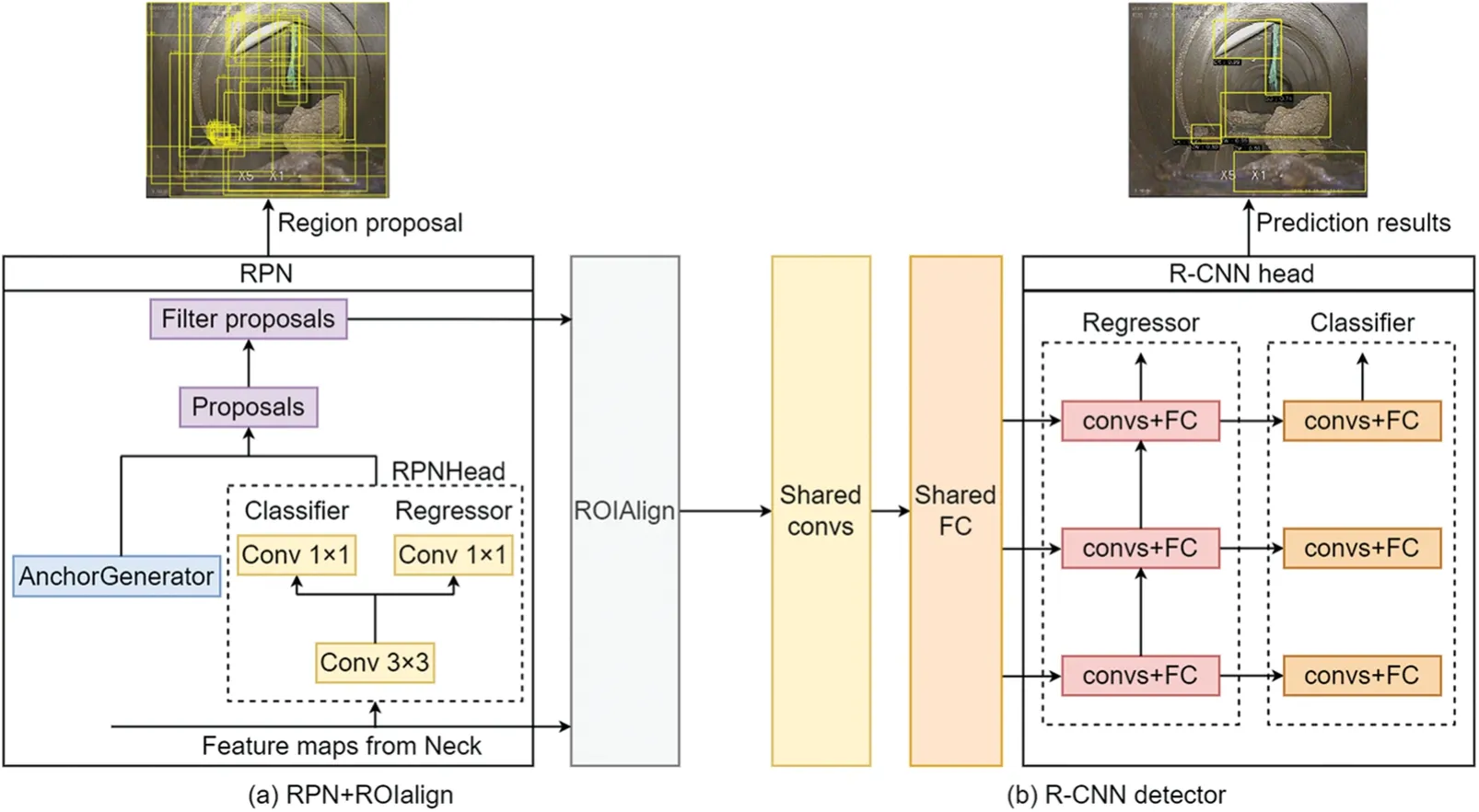
Figure 6:Structures of the RPN module and the R-CNN detector module

The RPN loss,consisting of the classification loss and the regression loss,is used to train the RPN module,as given by Eq.(3):

wherepiis the predicted probability of anchor is being an object,andpi∗is the corresponding groundtruth label,with 1 being a positive sample and 0 being a negative sample.Variabletiis a vector for the coordinates of the predicted bounding box,whileti∗represents its ground truth.NclsandNregare two normalization factors for the two components and are weighted by a balancing parameterλ,which is set to 1 for RPN loss.Lclsis the cross entropy loss for predictions on whether the region proposals are foreground or background.Lregis smooth L1 loss,as given by Eq.(4):

With the prediction from the RPNHead,only a small number of anchors that are likely to contain a defect will be provided for ROIAlign and the R-CNN detectors.

2.4.2 Cascade R-CNN Detector

For the multi-stage optimization approach,the output of the R-CNN detector in the current stage is used as the input of the R-CNN detector in the next stage to gradually optimize the quality of the prediction results,as shown in Fig.6b.During training,a detector randomly selects 512 samples from its preceding detector.Positive samples are determined based on the IoU between the ground truth bounding box and the predicted bounding box exceeding the training threshold.During testing,the cascade mechanism is also employed to iteratively refine the quality of predicted boxes.

Each detector’s loss function comprises two components: the regressor and the classifier,as depicted in Eq.(5).The loss function for the detector at stage t is defined as follows:

wherehtis a classifier,f tis a regressor at stage t,bt=f t-1 (xt-1,bt-1),g is the ground truth object forxt,ytis the classification label forxt,λis the trade-off coefficient.LCLSis cross-entropy loss andLlocis CIoU loss,which is introduced in[20].

2.5 Model Ensemble

The result from our architecture can be fused with others to further improve the accuracy.At the end of this architecture,inspired by[21],we have merged the prediction boxes based on different sewer defect detection model results.For each model,the prediction boxes are sorted according to their confidence scores.Starting from the prediction box with the highest confidence,other boxes whose IoU exceeds a certain threshold are assigned to the same cluster.For each cluster,the coordinates,confidence and classification of the weighted average are calculated and output as the final predicted box.The process is repeated until all of the boxes have been assigned and output.

3 Experimental Validations

3.1 Experimental Setup

CCTV inspection is used to obtain sewer interior videos in three Chinese cities: Zhongshan,Zhuhai,and Suqian.A total of 6756 images are captured as the dataset.The dataset consists of both concrete and plastic pipe and includes 9 classifications of defects:Mismatch(CK),Deposition(CJ),Deformation(BX),Root(SG),Disjointed(TJ),Concealed Joint(AJ),Cracking(PL),Barrier(ZW),and Foreign body penetration(CR).The number of corresponding defect samples is 3286(CK),1698(CJ),700 (BX),1052 (SG),454 (TJ),1957 (AJ),386 (CR),1393 (PL),1127 (ZW),respectively.In addition to the nine defect classes,969 normal class images(zc)were added to the dataset.All images in the dataset have been labeled with ground truth boxes.The model trained on the dataset can classify normal and defective images and locate the sewer defects.

All images have been annotated using the Labelme software,which annotates each sample with bounding boxes and class labels.These annotations are stored in corresponding XML files for each image.

In this study,80% of the dataset is allocated for training,while the remaining 20% is used for testing.Within the training set,10% of the data is reserved as a validation set for tuning model hyperparameters.

To fairly compare the model performance,we used MMDetection[22],which contains the SOTA object detection model,and MMYOLO [23],which contains YOLO’s overall method,for model training and evaluation.All experiments were conducted using models developed with PyTorch on a Windows 10 system with an Intel Xeon Silver 4208 central processing unit(CPU)running at 2.10 GHz and an NVIDIA RTX A8000 graphics processing unit(GPU).

3.2 Performance Evaluation

The mAP and mean Average Recall(mAR)are used to evaluate the detection performance of the model.These metrics are calculated based on precision and recall that are given below:

True Positive(TP)and False Positive(FP)are determined by IoU between the predicted bounding box and the ground truth bounding box with the following:

If the IoU exceeds a predefined threshold,the predicted bounding box is considered a TP sample.If it is less than the threshold or the predicted defect is incorrect,the predicted bounding box is counted as an FP sample.If there is no corresponding predicted bounding box,a False Negative(FN)will be counted.

The average precision(AP)is determined by calculating the mean of the highest precision values across various recall levels using Eq.(9):

wherep(r’)is the precision when the recall isr’,and M is the total number of TP.The mAP is calculated with the following,which is the average AP of all defect classes:

whereNclsis the number of defect classes in the dataset,andAPiis the AP for defect class i.

To assess the model’s recall performance,we compute the first 100 predicted bounding boxes per image.The average recall is denoted as AR,and the mean AR across all defect classes is referred to as mAR.

Two IoU thresholds are used in this work.When the IoU threshold is set to the average value from 0.5 to 0.95 with a step of 0.05 ([0.5:0.95]),this criterion requires a higher degree of precision in localizing the prediction box.When the IoU threshold is 0.5,this criterion lowers the demand for precise localization of the prediction box.

Four indicators are used to evaluate the model size,computational cost and speed of the model:model parameters,the floating point operations(FLOPs),GPU hours to complete one epoch during training and frames per second(FPS)during inference.

3.3 Model Training

3.3.1 ImageNet Pretraining of the Composite Backbone

The assisting Swin Transformer and the lead Swin Transformer can be initialized using the same pre-trained weights.Each Swin Transformer is pretrained for 90 epochs on ImageNet22k[24]with 224×224 images using AdamW[25].Other configurations are referenced in[11].

3.3.2 Fine-Tuning on the Sewer Dataset

Here a combination optimizer of AdamW and Stochastic Weight Averaging(SWA)[26]is used to optimize the model.AdamW is used as the first optimizer to train 15 epochs and SWA optimization is used for further optimization after AdamW to train 8 epochs.

The model’s loss curve,the mAP@[0.5:0.95]curve and the mAP@0.5 curve are shown in Fig.7.The most SWA training stage has higher losses than the later stage of AdamW training.Although the mAP also decreases slightly at the beginning,it increases rapidly later.This phenomenon occurs because there is a certain offset between training loss and test mAP,and SWA is not looking for a locally optimal solution but for a relatively flat region.

Figure 7:The(a)loss curve,(b)mAP@[0.5:0.95]curve,and(c)mAP@0.5 curve before and after using the SWA algorithm on the validation dataset.The left side of the dashed line indicates the model is optimized using AdamW,while the right side shows the model is optimized using the SWA

3.4 Ablation Study

Since our model consists of many optimized components and algorithms,we conduct ablation experiments,where each component will be compared with existing corresponding techniques.

The ablation experimental results of our model are given in Table 1.The results show that CBSwin outperforms the Swin Transformer in terms of both mAP and mAR.

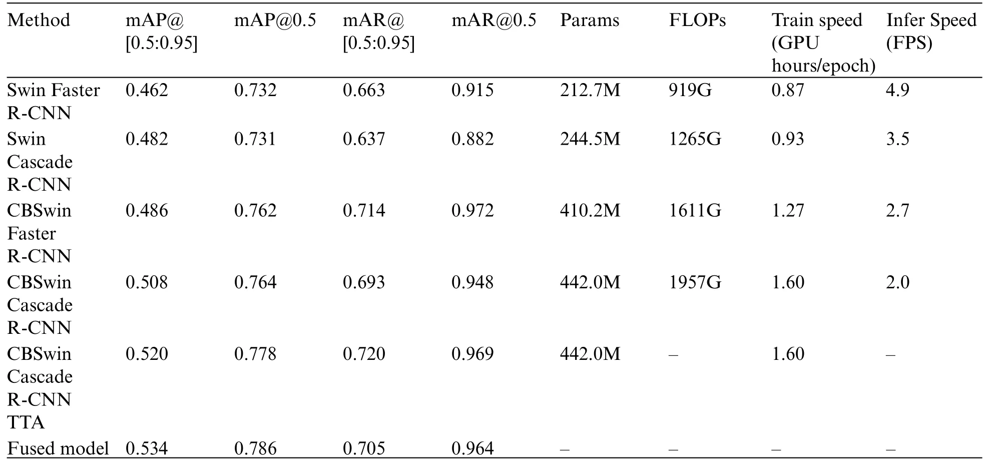
Table 1:Performance comparison of different models with IoU=[0.5:0.95]and IoU=0.5 criteria.Where Swin is the Swin Transformer;1 GFLOP indicates 1 billion floating point operations;The input resolution for all models is 800×1344 during inference.The fused model is the result of the fusion of the above four models

We also compare the two detectors: Faster R-CNN and Cascade R-CNN.The results show that the Cascade R-CNN achieves 50.8% and 76.4% under mAP@[0.5:0.95] and mAP@0.5 metrics respectively,which outperforms the Faster R-CNN.Cascade R-CNN has better recall performance than Faster R-CNN under the mAR@[0.5:0.95] metric.Under the mAR@0.5 metric,the recall performance of the two detectors is comparable.This reflects the fact that the cascade optimized detection allows the model to achieve better performance in sewer defect detection.

CBswin and Cascade R-CNN lead to an increase in the number of parameters and computational effort,and a decrease in training and inference speed.Nevertheless,it also shows that our model can effectively utilize more parameters to improve the generalization ability.

At test time,the original image is augmented to multiple sizes.The model ensembles the results for both the horizontally flipped images and the different image sizes.As shown in Table 1,TTA can significantly improve the mAP and mAR in sewer defect detection by 1.2% and 1.4% under mAP@[0.5:0.95]and mAP@0.5 metrics,and by 2.7%and 2.1%under mAR@[0.5:0.95]and mAR@0.5 metrics,respectively.

We fused the results of four transformer-based object detectors based on the above model.TTA was used for each model.The IoU threshold for fusion is set to 0.65 and the results are shown in Table 1.It can be seen that the model fusion operation can merge the bounding boxes of different models into a more accurate bounding box,which benefits the precision of object detection.The mAP after model fusion is 53.4%and 78.6%at mAP@[0.5:0.95]and mAP@0.5,respectively.However,at the same time,since model fusion predicts the average bounding box based on the confidence scores of all the proposed bounding boxes,some real defects may be incorrectly merged,which may not completely cover the original defects,thus reducing the mAR.

Visual Object Classes(VOC)[27]and roadsign datasets[28]are adopted to verify the generalization of the proposed method.The VOC dataset includes VOC2007 and VOC2012,which has a total of 20 classes,8218 training set images,8333 validation set images and 4952 test set images.The Roadsign dataset has 4 classes and 877 images,which is divided using the same proportions as the Sewer dataset.The detection results are shown in Table 2.It can be seen that CBSwin Cascade R-CNN outperforms Swin Faster R-CNN by 6.7% and 2.6% under mAP@[0.5:0.95] and mAP@0.5 metrics and by 5.9%and 2.9%under mAR@[0.5:0.95]and mAR@0.5,metrics on the VOC dataset,respectively.Even on a small dataset such as roadsign,CBSwin Cascade R-CNN also has good detection performance.This shows that CBSwin Cascade R-CNN can detect and recognize different classes of objects more accurately.

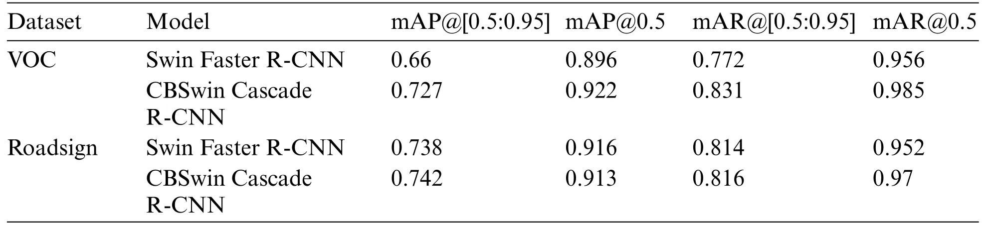
Table 2: The performance of our model on the VOC and roadsign datasets

3.5 Full-Fledged Study

3.5.1 Comparison with Other Object Detection Methods

We have compared our CBSwin Cascade R-CNN model with other advanced object detection methods,and the results are shown in Table 3.CBSwin Cascade R-CNN has the highest mAP and mAR,indicating that it has great performance and robustness in the sewer object detection task.The Precision-Recall curve is plotted to measure the accuracy and recall of the models.We uniformly take 101 precision values from the corresponding 101 recalls from 0 to 100 when the IoU threshold is 0.5,and take the average of the precision values for the 10 defect classes.The larger the area between the Precision-Recall curve and the coordinate axis,the better the model performs on the imbalanced dataset.It can be seen that the area enclosed by the Precision-Recall curve of our model is significantly larger than those of the other eight models,indicating that the performance of our architecture for sewer object detection is the best,as shown in Fig.8a.

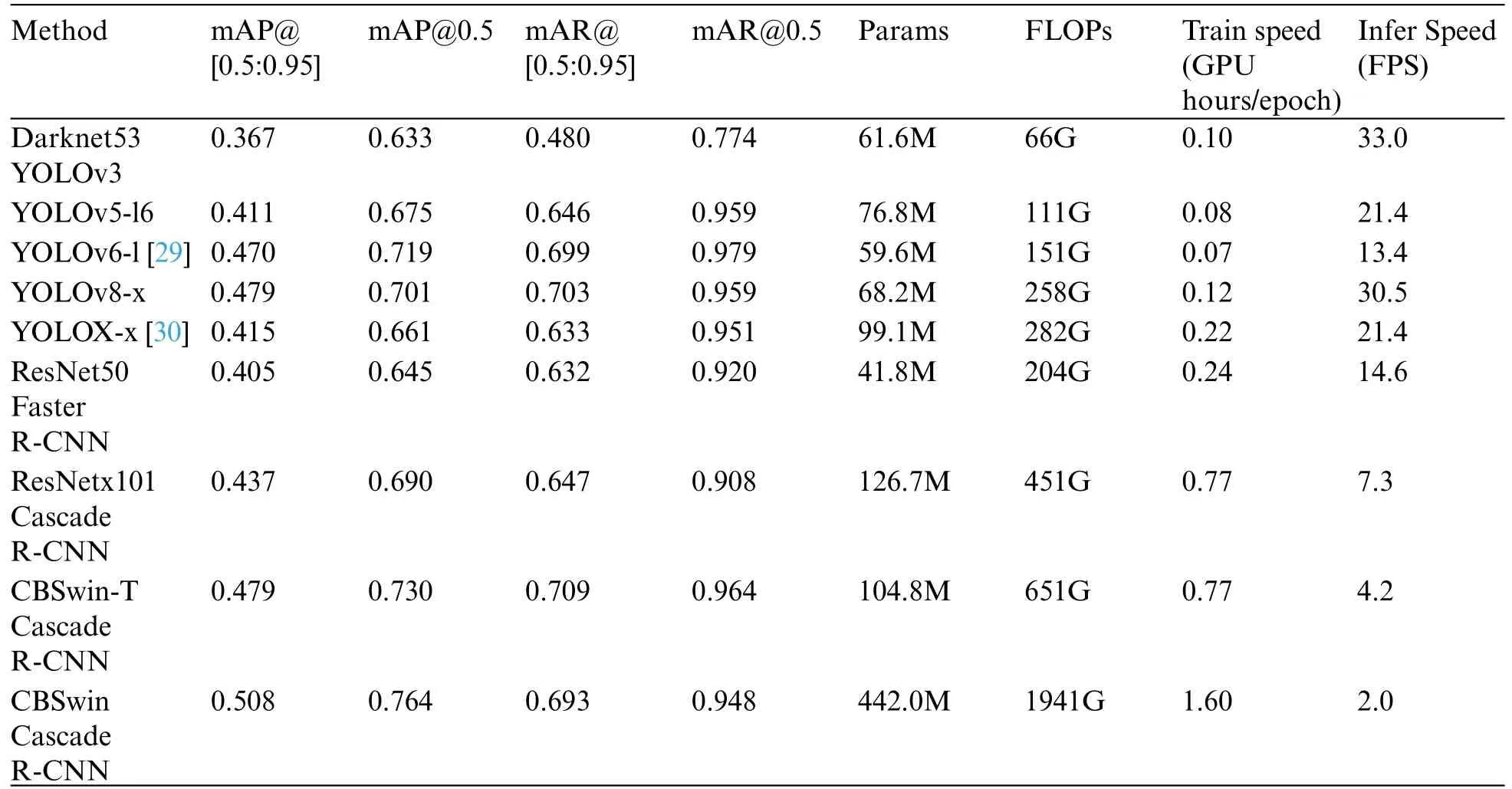
Table 3:Comparison of our model with other advanced object detection models in the test dataset.All YOLO models are trained for 300 epochs and R-CNN models are trained for 23 epochs.The input resolution for YOLOv3 is 416 × 416 and for the other YOLO models,it is 640 × 640.The input resolution for all R-CNN models is 800 × 1344.Other hyperparameters are adopted as the default setting in the MMDetection and MMYOLO

Each Swin Transformer is compressed to a tiny size(CBSwin-T Cascade R-CNN)and compared with the CNN structures.It can be found from Table 3 that with the less model parameters,the composite backbone transformer can make the model achieve higher mAP and mAR than other CNN models.Although CBSwin-T Cascade R-CNN has the highest mAP compared to YOLO,it has a disadvantage in speed and computational complexity.The CBSwin Cascade R-CNN is larger and slower than other models,but the current sewer defect detection and subsequent repair are different processes,so there is no need to directly evaluate the sewer defect detection on-site and obtain immediate results.Our algorithm should be placed in the cloud or on the computers of in-house data personnel to assist them in swiftly evaluating defects,thereby reducing their workload in generating reports.In this case,the CBSwin Cascade R-CNN model will give more accurate results to professional engineers.

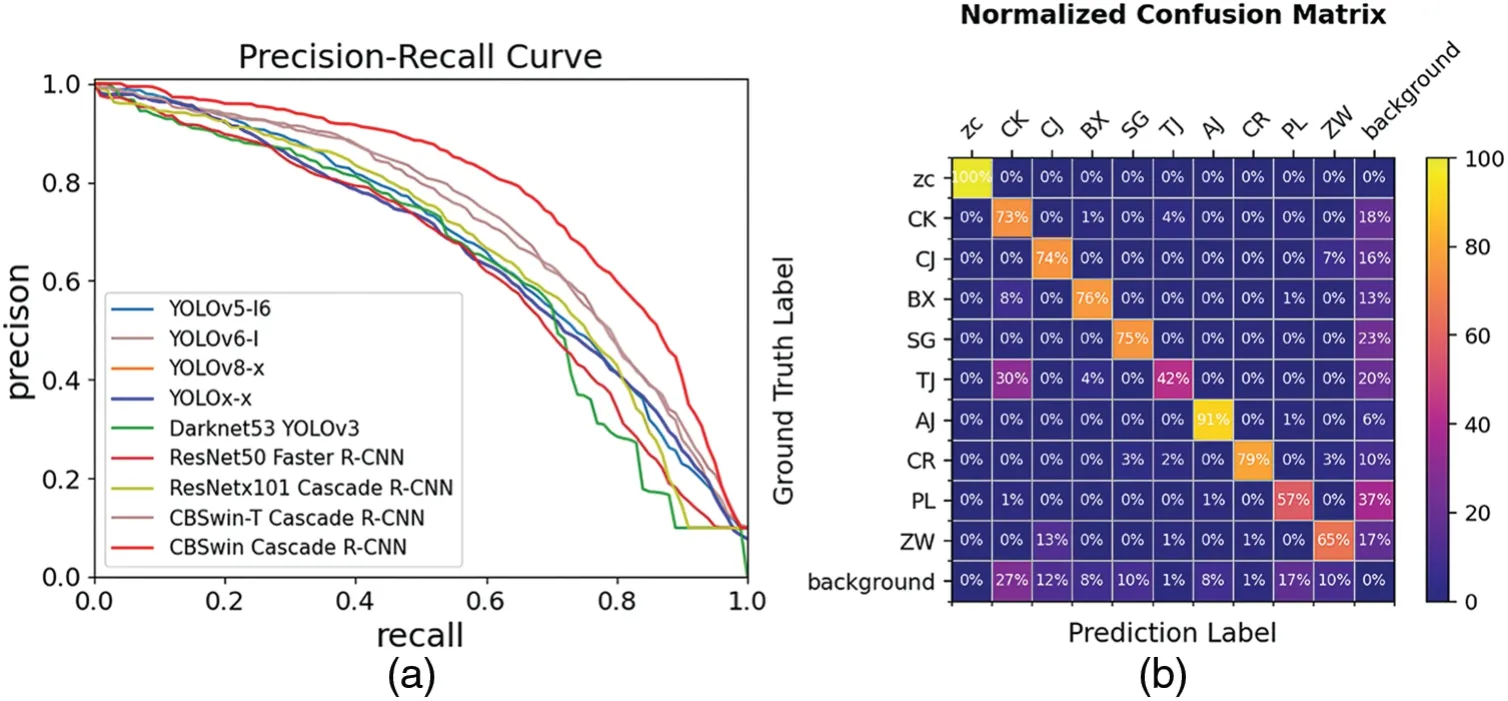
Figure 8: Confusion matrices of (a) Comparison Precision-Recall curves of five other models.(b)CBSwin Cascade R-CNN with TTA

3.5.2 Performance of the Model for Each Defect Classes

The mAP and mAR for each class of defect are shown in Table 4 and the percentage confusion matrix of our model is shown in Fig.8b.The rows of the matrix are ground truth labels,and the columns of the matrix are predicted labels.The diagonal direction of the matrix shows the TP for each class.The last column of the matrix shows the FN and the other columns show the FP.It is shown that our model can filter out almost all normal images and has good detection performance for most defect classes.However,due to the limited feature pixels of the PL class,it results in relatively poor detection of the PL class with the model.Due to the similarity of features,some TJ classes are easily misclassified as CK classes.These issues will be our future research direction.

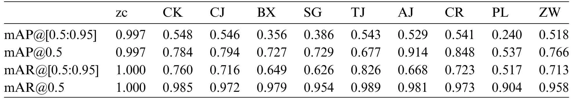
Table 4: The performance of our single model for each classification in the test dataset

4 Conclusions and Future Work

Sewer defect detection is a special kind of anomaly detection.The success of deep learning-based anomaly detection can be effectively applied to sewer defect detection,as evidenced by numerous recent efforts in this area.However,previous work has certain limitations,primarily in the dataset’s coverage of specific defect classes,resulting in a restricted detection capability for these classes using the proposed models.In this paper,a dataset consisting of a variety of different sewer defects that can cover a wide range of situations that may occur in real sewer pipes has been collected.A novel composite transformer-based multi-stage sewer defect detection model has been proposed and trained on the sewer defect dataset.Experiments show that the composite backbone,the multistage detector and the test-time data augmentation can significantly influence the architecture’s performance.Our architecture achieves a performance of 52.0%and 77.8%under mAP@[0.5:0.95]and mAP@0.5 metrics,respectively,where the composite backbone Swin Transformer module improves the performance most significantly.After model fusion,the model achieves 53.4%and 78.6%under mAP@0.5 and mAP@[0.5:0.95]metrics.When compared to alternative sewer object detection models,our model shows outstanding generalization capabilities.In addition,our model is more suitable for defect detection in the cloud or on the computers of in-house data personnel.

In our future work,we will focus on the detection of challenging samples,particularly by improving the mAP in localizing PL defects.Additionally,we will address the issue arising from varying shooting angles,where TJ defects may be prone to misdiagnosis as CK defects.

Acknowledgement:Not applicable.

Funding Statement:This work was supported by the Science and Technology Development Fund of Macau (Grant No.0079/2019/AMJ) and the National Key R&D Program of China (No.2019YFE0111400).

Author Contributions:Conceptualization,Methodology,Writing—original draft,Writing—review&editing:Z.Yu;Principal investigator,Design of the framework,Writing—review&editing,Supervision:X.Li;Data analysis:L.Sun;Data collection and labeling:J.Zhu;Data collection,labeling and analysis:J.Lin.All authors reviewed the results and approved the final version of the manuscript.

Availability of Data and Materials:The source code and the demo video for the paperwork are available at https://github.com/ZF-Yu/Sewer-defect-detection.The data sets used in this work are available upon request.

Conflicts of Interest:The authors declare that they have no conflicts of interest to report regarding the present study.