Using MsfNet to Predict the ISUP Grade of Renal Clear Cell Carcinoma in Digital Pathology Images

Kun Yang ,Shilong Chang ,Yucheng Wang ,Minghui Wang ,Jiahui Yang ,Shuang Liu ,Kun Liu and Linyan Xue,⋆

1College of Quality and Technical Supervision,Hebei University,Baoding,071002,China

2National and Local Joint Engineering Research Center of Metrology Instrument and System,Hebei University,Baoding,071002,China

3Hebei Technology Innovation Center for Lightweight of New Energy Vehicle Power System,Hebei University,Baoding,071002,China

ABSTRACT Clear cell renal cell carcinoma (ccRCC) represents the most frequent form of renal cell carcinoma (RCC),and accurate International Society of Urological Pathology (ISUP) grading is crucial for prognosis and treatment selection.This study presents a new deep network called Multi-scale Fusion Network (MsfNet),which aims to enhance the automatic ISUP grade of ccRCC with digital histopathology pathology images.The MsfNet overcomes the limitations of traditional ResNet50 by multi-scale information fusion and dynamic allocation of channel quantity.The model was trained and tested using 90 Hematoxylin and Eosin(H&E)stained whole slide images(WSIs),which were all cropped into 320 × 320-pixel patches at 40× magnification.MsfNet achieved a microaveraged area under the curve (AUC) of 0.9807,a macro-averaged AUC of 0.9778 on the test dataset.The Gradient-weighted Class Activation Mapping(Grad-CAM)visually demonstrated MsfNet’s ability to distinguish and highlight abnormal areas more effectively than ResNet50.The t-Distributed Stochastic Neighbor Embedding(t-SNE)plot indicates our model can efficiently extract critical features from images,reducing the impact of noise and redundant information.The results suggest that MsfNet offers an accurate ISUP grade of ccRCC in digital images,emphasizing the potential of AI-assisted histopathological systems in clinical practice.

KEYWORDS Renal cell carcinoma;computer-aided diagnosis;pathology image;deep learning;machine learning

1 Introduction

Renal cell carcinoma (RCC) is the predominant kidney cancer,comprising about 3% of all cancer cases,with a 2%increase in annual incidence worldwide[1].There are three major histological subtypes of RCC (chromophobe cell carcinoma,clear cell carcinoma,and papillary cell carcinoma)that histological and clinical alterations can differentiate.Among them,the most common and lethal one is the ccRCC,which is reported to be 80% of RCC cases [2].For ccRCC patients,microscopic tissue analysis continues to be the gold standard for diagnosis,and accurate assessment of cancer grading increases their chances of successful treatment[3].However,conventional manual pathology examination requires a high workload,and the subjective grading assessment inevitably leads to inconsistency among pathologists.Consequently,a more reliable tool for rapid and accurate pathological diagnosis of ccRCC is urgently needed.

In recent years,the integration of computer-aided diagnostic (CAD) systems into medical pathology has significantly advanced the analysis of histopathological images across a variety of organspecific cancers,including those of the breast[4],kidneys[5],prostate[6],stomach[7],and colonoscopy[8].These systems have been employed in a range of tasks,such as the detection and segmentation of cell nuclei,as well as the characterization and grading of cancer subtypes[9].

Despite the broad application of CAD,the automation of RCC pathology image diagnosis has concentrated on elementary grading and typing,in addition to prognostic predictions.Zheng et al.[10]introduced a deep learning multi-class model,SSL-CLAM,designed to assist in determining the Furman grade status of ccRCC patients.This model was trained and validated on 708 digitized WSIs from 504 patients,demonstrating superior performance in the binary classification of Furman grades,with AUC scores of 0.936 and 0.915 for internal and external validation sets,respectively.Fenstermaker et al.[11]explored the efficacy of a Convolutional Neural Network(CNN)in identifying the presence of RCC in histopathology specimens and in differentiating between RCC subtypes and grades.The CNN model achieved a remarkable overall accuracy of 99.1% in the testing cohort,with a sensitivity of 100% and specificity of 97.1% for RCC detection.It also demonstrated a 97.5% accuracy in subtype differentiation and a 98.4% accuracy in Fuhrman grade prediction.Haeyeh et al.[12]proposed a novel multiscale,weakly-supervised deep learning framework for RCC subtyping,which distinguished between benign and malignant RCC tissues and accurately identified tumor subtypes,thereby facilitating medical therapy management.This system attained an overall classification accuracy of 93.0%±4.9%,with a sensitivity of 91.3%±10.7%and a specificity of 95.6%±5.2%for differentiating ccRCC from non-RCC tissues.Wessels et al.[13]assessed the capability of a CNN to extract pertinent features from hematoxylin and eosin-stained slides for predicting 5-year overall survival (5y-OS) in patients with ccRCC.The CNN,trained on TCGA slides and validated on an independent cohort,achieved a mean balanced accuracy of 72.0%,with a sensitivity of 72.4%,specificity of 71.7%,and an AUC of 0.75,when combined with clinicopathological parameters through multivariable logistic regression.

Despite the progress in RCC diagnostic and grading methodologies,significant challenges remain.The prevailing algorithms for pathological grading have not adequately captured the intricacies of ccRCC grading.A notable example is the reliance on the Fuhrman grading system,which is beset with issues of subjectivity and limited reproducibility,casting doubts on its diagnostic criteria and prognostic validity [14].Furthermore,some diagnostic models tend to oversimplify grading by classifying tumors into broad categories such as high-grade and low-grade,thereby lacking the granularity required for a detailed diagnosis.

This study introduces an enhanced CNN architecture,termed the Multi-Scale Fusion Convolutional Network (MsfNet),aiming to refine the pathological grading of ccRCC.This is achieved by improving feature extraction capabilities through an innovative approach that integrates and fuses information from various sampled inputs.The International Society of Urological Pathology(ISUP)grading system,which is recommended for prognostic prediction in ccRCC,stratifies tumors into four distinct grades [15].The ISUP system specifies that grades 1–3 are determined by the degree of nucleolar prominence,whereas grade 4 is distinguished by marked nuclear pleomorphism,the presence of giant tumor cells,and/or the manifestation of rhabdoid and sarcomatous differentiation.Consequently,there is a potential for inter-observer variability in the classification of tumors into grades 1–3,though grade 4 typically presents more definitive features.

To address this variability and to provide a more objective measure in the differentiation of benign and malignant tissue,as well as to diminish the inter-observer variability,particularly among ISUP grades 1,2,and 3,this paper proposes a novel,computer-aided approach.The aim is to leverage the MsfNet to establish a consistent and reproducible grading mechanism that can support pathologists in making precise and reliable assessments of ccRCC.

A total of 90 pathological slice Images of renal tissue were collected from Zhongke Guanghua(Xi’an) Intelligent Biotechnology Co.,Ltd.(China),of which 80% were training dataset,and 20%were test dataset.Owing to the exceptionally large size at 40×magnification,the pathological images in the training set and test set were cut into 19,963 patches,the size of every patch is 320 × 320.Experimental results show our proposed method achieved 0.9807 micro-averaged AUC and 0.9778 macro-averaged AUC.

In short,our contributions are summarized as follows: (1) A novel MsfNet is established using multi-scale feature fusion and channel reweighting,which achieves state-of-the-art classification performance on the task of ccRCC grading in pathological images.(2) This study explores the use of deep learning to assist pathologists,providing a possible joint diagnosis mode,which illustrates its potential for clinical treatment and prognostic assessment.

The remainder of this paper is organized as follows.Section 2 presents the related work of this study.Section 3 provides the detailed description of the model proposed in this paper.Section 4 describes the datasets used in the experiments and the data processing procedures.Section 5 presents the experimental results and analysis.Finally,Section 6 concludes the content of the paper and provides directions for further research.

2 Related Work

The examination of WSIs is a labor-intensive process that is subject to considerable variability among pathologists,underscoring the critical need for the development of CAD systems.These systems aim to automate and enhance the reliability of the analysis of H&E-stained histopathological images.Current CAD methodologies predominantly pivot on two paradigms: Machine Learning(ML)and Deep Learning(DL)[16].

Machine learning-based CAD systems typically require the manual extraction of features,such as textural and morphological attributes,which are then utilized to construct classifiers,such as Support Vector Machines(SVM),Random Forests(RF),and K-Nearest Neighbors(K-NN),for subsequent classification or regression tasks.For instance,Moncayo et al.[17] in 2015,introduced a machine learning framework for breast cancer grading that employed SVM classifiers to analyze alterations in nuclear size,shape,and chromatin texture.This approach was validated on 134 fields of view(FOVs)at 20×magnification,extracted from 14 breast cancer slides from the Cancer Genome Atlas(TCGA) database,with the grading performed by a pathologist.The method achieved an accuracy and recall rate of 0.67.Rathore et al.[18] extracted a combination of clinical and imaging features,including both conventional (intensity,morphology) and advanced textural features (gray-level cooccurrence matrix and gray-level run-length matrix),from WSIs.These features were employed to train an SVM model with a linear configuration,which was then validated on glioma patients with a 10-fold cross-validation,achieving an accuracy of 75.12%and an AUC of 0.652.Kruk et al.[19]utilized an ensemble of classifiers in conjunction with wavelet transformations to enhance the recognition of Fuhrman grading in ccRCC,achieving a sensitivity of 94.3%and a specificity of 98.6%,which marked a significant improvement over the existing result.Humphrey et al.[20] leveraged machine learning with an SVM to predict early recurrence of hepatocellular carcinoma (HCC) post-resection,using digital pathological images from 158 HCC patients.The model demonstrated an accuracy of 89.9%,suggesting that digital pathology combined with machine learning can be a potent tool for the accurate prediction of HCC recurrence,particularly in early stages post-surgery.

While ML methodologies have demonstrated utility in the analysis of medical pathological images,they are not without limitations.These approaches necessitate a considerable degree of expertise and often require extensive preprocessing of image datasets to extract pertinent features.This preprocessing is a critical step,as the performance of ML algorithms is heavily dependent on the quality and relevance of the features extracted.In contrast,DL represents a data-driven paradigm that has revolutionized medical image analysis,particularly due to its superior performance in image classification tasks.DL algorithms,particularly CNNs,have the ability to automatically learn hierarchical feature representations from raw data,which is a significant advantage over traditional ML techniques.

Recent research has underscored the efficacy of DL in the domain of medical pathological image analysis.Baris et al.[21]improved a model based on MatConvNet to classify WSIs of breast biopsies into diagnostic categories,achieving an accuracy of 55% across five distinct color-coded categories.Thomas et al.[22] implemented a U-Net-like decoder architecture in their CNN classifier,which attained a high classification accuracy of 93.6% across various skin cancer grades using a dataset magnified 10 times.Lin et al.[23] employed a GoogleNet-based binary classifier for hepatocellular carcinoma histopathology images,which yielded an accuracy of 91.37%,with a sensitivity of 92.16%and a specificity of 90.57%.Jaber et al.[24] utilized the Cox proportional hazards model to stratify the risk in negative breast cancer patients,demonstrating that their method improved risk prediction over traditional baseline models through the analysis of 506 images,including WSIs and hormone receptor statuses.Wessels et al.[25]developed and validated a vision transformer(ViT)using a selfsupervised learning model,DINO (self-distillation with no labels),to predict overall survival (OS)and disease-specific survival(DSS)in ccRCC,with the DINO-ViT risk stratification proving to be a significant predictor for both OS and DSS.Lastly,Sun et al.[26] proposed a hybrid multi-instance learning model,TGMIL,combining the Transformer and the Graph Attention Network to classify WSIs of RCC.This model achieved impressive AUC and accuracy rates on a public dataset for RCC,without the need for pixel-level annotation or region of interest extraction.

3 Methods

3.1 Convolutional Neural Network

CNN is one of the most frequently adopted deep learning approaches,as its hierarchical structure with multiple layers yielded state-of-the-art performance in classification and detection tasks,such as energy forecasting [27],new materials [28],and intelligent medicine [29].To learn numerous levels of abstraction for data representation,a CNN mainly encompasses three types of layers:(i)convolutional layers,applying kernel filters to extract features from input images;(ii)pooling layers,using statistical information(max,mean,etc.)substituting small feature map neighborhoods with to reduce spatial resolution;and (iii) activation layers,employing activation functions on feature maps(typically elementwise)to facilitate the non-linear model[30].

In recent years,a variety of backbone network variations have been introduced and refined for learning in CNNs.For instance,LeNet[31]uses a back-propagation algorithm as an early successful gradient learning example.AlexNet [32] is a pioneering deep architecture with an 84.6% top-5 test accuracy on ImageNet data.VGGNet[33]demonstrates significant improvements by pushing depth to 16–19 weight layers in large-scale image recognition settings.ResNet[34]introduces a residual learning framework to facilitate the training of substantially deeper networks than before.

3.2 Multi-Scale Fusion Residual Network

Most previous methods enhance the performance by increasing the network depth and using filters with smaller kernel sizes.In our study,an improved residual network architecture based on ResNet,namely MsfNet,was developed to improve the feature extraction ability of the proposed network by fusion of multi-scale features.

The proposed pipeline is shown in Fig.1.Our model’s structure design is adopted from the ResNet50 design and is built using the Pytorch backend.The main structure of ResNet50 is composed of 5 stages,followed by a 4-way fully connected layers (denoted as fc-layer in Fig.1a) and a final softmax layer.Except that the first stage includes a 7 × 7 convolution layer and a 3 × 3 maxpooling layer,the other stages contain several bottleneck blocks in respective order(see Fig.1a).As a basic component module in many of the backbone networks,the bottleneck blocks employed in our proposed network extract features from the pathology images and update weights during training.In a more concise manner,Stages 2 to 5 contain 3,4,6,and 3 bottleneck blocks each.The bottleneck block comprises three convolution kernels:(1)a 1×1 kernel that reduces input channels to 1/4,minimizing computational load;(2)a 3×3 kernel for feature extraction;and(3)a final 1×1 kernel that restores the channel count to its initial amount.The residual link between input and output functions as an identity map,enabling feature map inheritance from previous blocks and facilitating deep network training.Additionally,by using a global average pooling layer(GAP)and a 4-way fully connected layer with softmax,the network outputs a 4-dimension tensor which represents the predicted probabilities of each ccRCC ISUP grade.The grade with the max probability is decided as the final prediction result of the network.

Figure 1: The network structures of ResNet50 and the proposed MsfNet.(a) Pipeline of ResNet50;(b)Pipeline of our proposed MsfNet

While ResNet allows for considerably deeper,more accurate,and more efficient training through shorter connections between input-proximate and output-proximate layers,it may sacrifice original shallow semantic information during deeper feature extraction.For achieving more representation at each scale of both the shallow and deep semantic information from input patches,a multi-scale information fusion residual network was integrated into ResNet50 to aggregate featuresx1,x2,x3,x4,and x5,which output from different stages with different semantic depths.Specifically,as shown in Fig.1b,our method MsfNet has two significant differences from ResNet50.

Multi-scale information fusion:For more efficient feature extraction,the output at anywhere stage incorporates multiple inputs from all preceding stages and repeated use for further feature aggregation in subsequent stages,rather than solely considering the input feature map from the immediately preceding layer.

Fig.1b illustrates the workflow of the proposed network schematically.It can denote the feature map generated by stagesthasxs∈RW×HXC,W,HandCrepresent the width,height,and channel dimension of the feature map,respectively.In traditional ResNet architecture,the representationxsis then directly passed to the following stage as the input of the(s+1)thstage,which can be represented by

It should be noted thatI6represents the input feature map of the fc-layer.However,this type of connection between individual layers only obtains feature representation from a particular stage,leading to the limitation of information flow in subsequent stages.In the proposed MsfNet,stage interconnections are generated utilizing preceding feature representations for aggregating features from various receptive regions.The operation is initially performed by downsampling different scale feature maps to uniform spatial resolutions.Following that,these downsampled variants of feature maps are integrated into a fusion feature vector,which is achieved by using multiple inputs from all preceding stages to create a feature map,and then repeatedly employed for further feature aggregation in subsequent stages.Afterward,the fusion vector and the shortcut connection are aggregated through concatenation and are passed through the following stage.The fusion of feature vectors can be represented as

where theis the output feature map from theithstage to be fused with the feature map ofxsin thesthstage withcnumber of channels.

Dynamic allocation of channel quantity:At the same time,considering that the feature maps output at different stages contains different levels of semantic information.Inspired by[35],while making full use of the shallow semantic information in order to ensure that the model can extract deeper feature information.As shown in Eq.(2),this study designed a simplified channel quantity allocation strategy,assigning more channel quantity to the feature maps with deeper semantic information while assigning less quantity to the shallow feature maps.In addition,to successfully complete the concatenate of feature maps,max pooling is applied to ensure that the feature maps have the same size,and then a 1×1 convolution is used to change the channel feature maps.

Take the input of Stage 4,which is denoted asI4,i.e.,the output of Stage 3 in ResNet50,as an example.In MsfNet,I4is the concatenation of the preceding stage output (x1,x2,x3).The specific process is as follows:firstly,the max-pooling with the kernel of 4 or 2 is used to ensurex1andx2have the same height and width asx3.Then,the feature mapare calculated by a 1×1 convolution which is used to assign different channels to the 1th,2th,and 3thstages,andandCare representative of the channel ofx33,x32,x31andx3.It should be noted thatrepresents the feature map obtained by processingx3,represents the feature map obtained by processingx2,represents the feature map obtained by processingx1.Finally,the fusion vectorare channel-wise additions with the feature mapx3through shortcut connection according to residual learning.Following that,Table 1 presents the structural details of all stages,which operate with different scales of feature maps in the fusion module.

Table 1:The detail of all stages operates with different scales of feature maps in MsfNet and ResNet50

4 Experiment

The workflow of the experiment is shown in Fig.2,which consists of 4 phases:data collection and preprocessing,data augmentation,model training,and performance test.

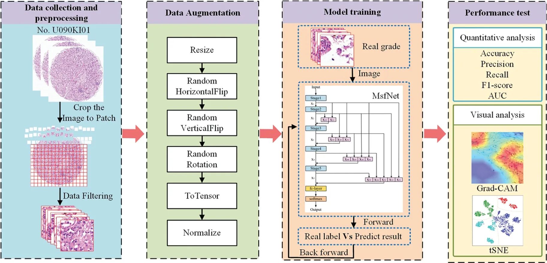
Figure 2:The workflow of the experiment about predicting the ISIP grade of ccRCC using MsfNet

4.1 Data Collection and Preprocessing

This study collected the renal tissue sections of 90 patients from the No.U090KI01 clear cell renal cell carcinoma tissue chip of Zhongke Guanghua(Xi’an)Intelligent Biotechnology Co.,Ltd.Of these,80 patients were diagnosed with clear cell carcinoma of the kidney,and 10 were diagnosed as normal.Table 2 presents the specific clinical characteristics of these patients:

In terms of data,this study is different from other scholars in that this study divided the data set by patients and divided 80%of patients into training set and 20%of patients into testing set according to the different diseases.The training set,which contains 31 ISUP I patients,22 ISUP II patients,13 ISUP III patients,and 8 normal patients,is used to participate in the iterative training of the model to get the best performance model.The testing set,which contains 7 ISUP I patients,4 ISUP II,3 ISUP III patients,and 2 normal patients,is used to test the performance of the network.

The original size of each pathological image was 5120 × 5120,and it is impossible to feed the entire pathological sections into the neural network at once.So,this work decided to cut pathological sections of each patient’s renal tumor at 40 times the microscopic magnification.As shown in Fig.2,firstly,cut the image into 320×320 pixels small patches.Meanwhile,in order to reduce the information loss,this study set the step size is 260.Then,filtered the cut patches and eliminated the ones that only contained blank areas,tissue fibers,bleeding,blood vessels,cysts,and lymphatic lesions that did not belong to cancer.The final training set has 16,547 image patches,and the testing set has 3,416 image patches.

4.2 Data Augmentation

Data augmentation is one of the important methods to improve network performance and reduce the risk of overfitting classification network models [36].Inevitably,the study has also conducted data augmentation processing on the filtered patches.The main training set process is illustrated in Fig.2.First,the patches are resized to 256 × 256 pixels.Subsequently,a set of transformation operations,including random horizontal flips,random vertical flips,random rotation of the image and normalization processing,are conducted.Finally,the resulting tensor is fed into the CNN model for training.However,for the testing set,the patches only need to be resized to 256×256 pixels and undergo normalization processing before being input into the CNN model.

4.3 Implementation Details of Model Training

To accelerate model training while improving generalization and stability,this study initialize ResNet weights using the ImageNet dataset[37].Every model was trained with 100 epochs,a batch size of 32,and optimized network parameters using the stochastic gradient descent(SGD)algorithm.The learning rate is 0.005 and decays to one-tenth of the original rate every 30 epochs.

4.4 Metrics of Performance Test

Firstly,the loss function uses the cross-entropy loss,and the calculation method,as shown in Eq.(3),xrepresents the input sample,yrepresents the actual label,˜yrepresents the predicted output,andnrepresents the total number of samples.

Then,to present the evaluation results,the label values were categorized into positive and negative.Finally,this study employed the metrics of Accuracy,Precision,Recall,and F1-score to quantitatively assess the model’s performance.Accuracy represents the prediction accuracy,determined by dividing the total number of correct predictions by the overall sample count.Precision represents the likelihood that a correct prediction is a positive sample among predicted positives.Recall denotes the probability that an original sample is correctly predicted as positive.F1-score serves as a harmonic mean evaluation index for precision and recall.

5 Results and Discussions

5.1 Ablation Analysis

This study compared the performance of ResNet50 and MsfNet with different structures,which used dynamic weight multi-scale feature fusion before the current stage,on the same testing set including 16,547 images from 17 patients.Different network structures are illustrated in Figs.1b and 3.Fig.3 illustrates different structures of MsfNet using dynamic weight multi-scale feature fusion strategy in the preceding stages.Taking Fig.3c as an example,‘stage=5’indicates that the feature vectors inputted in Stages 3,4,and 5 have all incorporated the dynamic weight multi-scale feature fusion proposed in this paper,while ‘stage=1’and ‘stage=2’signify that the input feature scales are single,without employing the multi-scale feature fusion strategy.

The corresponding results are shown in Table 3,where bold data represents the best results for each metric.As observed from Table 3,the performance of the MsfNet model exhibits a continuous improvement trend as the number of stages using dynamic weight multi-scale feature fusion increases.This provides validation for the effectiveness of dynamic weight multi-scale feature fusion and channel reweighting techniques.Particularly,when‘stage=6’is performed,indicating the application of dynamic weight multi-scale feature fusion to all input feature vectors,MsfNet achieves the best results across all metrics.MsfNet (stage=6) surpasses ResNet50 by 1.78% accuracy (87.06%vs.85.28%),1.61%precision(87.78%vs.86.17%),1.38%recall(85.85%vs.84.47%),and 1.83%F1-score(86.72%vs.84.89%).These results indicate that in the proposed network MsfNet,dynamic weight multi-scale feature fusion extracts additional valuable features from input images by preserving shallow visual information and incorporating deep semantic understanding.This substantially enhances the expression capability of the proposed network compared to the baseline ResNet50.

Table 3:Performance metrics comparison(%)between ResNet50 and MsfNet with different feature fusion structure

Then,in order to further compare the performance of the MsfNet and ResNet50,this work have drawn their receiver operating characteristic curve (ROC) and calculated the AUC.The ROC reflects the recognition ability of a classifier to samples at a certain threshold.The abscissa represents the false positive rate predicted by the classifier,while the ordinate represents the true positive rate predicted by the classifier.The AUC describes the overall discrimination ability of the classifier.The closer the curve is to the upper left corner,and the larger the area under the curve,the better the mode’s performance.Considering the problem of sample imbalance in the testing set and to more effectively assess the model’s performance,the macro-average and micro-average ROC curves of various algorithms are drawn,and the corresponding macro-average and micro-average AUC values are calculated,respectively.

As shown in Table 4,consistent with the results from Table 3,as more stages utilize dynamic weight multi-scale feature fusion,the performance of MsfNet improves.When‘stage=6’,except the MsfNet AUC value of discriminate normal pathological images is lower than ResNet50 (0.9957vs.0.9979),the MsfNet50 AUC value of micro-average (0.9807vs.0.99740),macro-average (0.9778vs.0.9707),ccRCC1(0.9811vs.0.9781),ccRCC2(0.9521vs.0.9351),ccRCC3(0.9818vs.0.9711)are better than ResNet50.The result shows that fusing the multi-scale feature and reusing the shallow semantic information is effective for MsfNet to achieve better performance than the baseline ResNet50.

Table 4: Comparison of the AUC values of ResNet50 and MsfNet with different structure

5.2 Visual Analysis

This study introduced Grad-CAM to intuitively observe the change in the region of interest(ROI)of the improved model when outputting the predicted result of the input image.The Grad-CAM[38]generates a coarse localization map by utilizing the gradient of a target concept flowing into the final convolution layer,highlighting crucial regions in the image for concept prediction.Because the classifier predicts the grade of the pathological image according to the morphology of cell nucleolus,if the ROI of the network is more concentrated with the nuclear region,it can extract more useful classification features and eliminate the interference of irrelevant regions.

In Fig.4,three types of pathological images of(a)mixed cancelation area and blank area,(d)all are cancerous regions,and(g)all are normal regions to observe the changes of the concerned regions of the ResNet50 and the improved network MsfNet,respectively.Figs.4b,4e and 4h are the Grad-CAMs of the ResNet50 produced from images Figs.4a,4d,4g,and Figs.4c,4f,4i are the Grad-CAMs of the MsfNet produced from images in Figs.4a,4d and 4g.Compared with ResNet50,the focus on the feature area of MsfNet is more accurate,and the effect is significantly improved.The visualized results show that the MsfNet can focus on more important areas in the pathological image patches to predict ISUP grade.This can be explained by the fact of the weighted fusion of the multi-scale feature map extract by different stages and reusing the shallow semantic information and the deep semantic information.

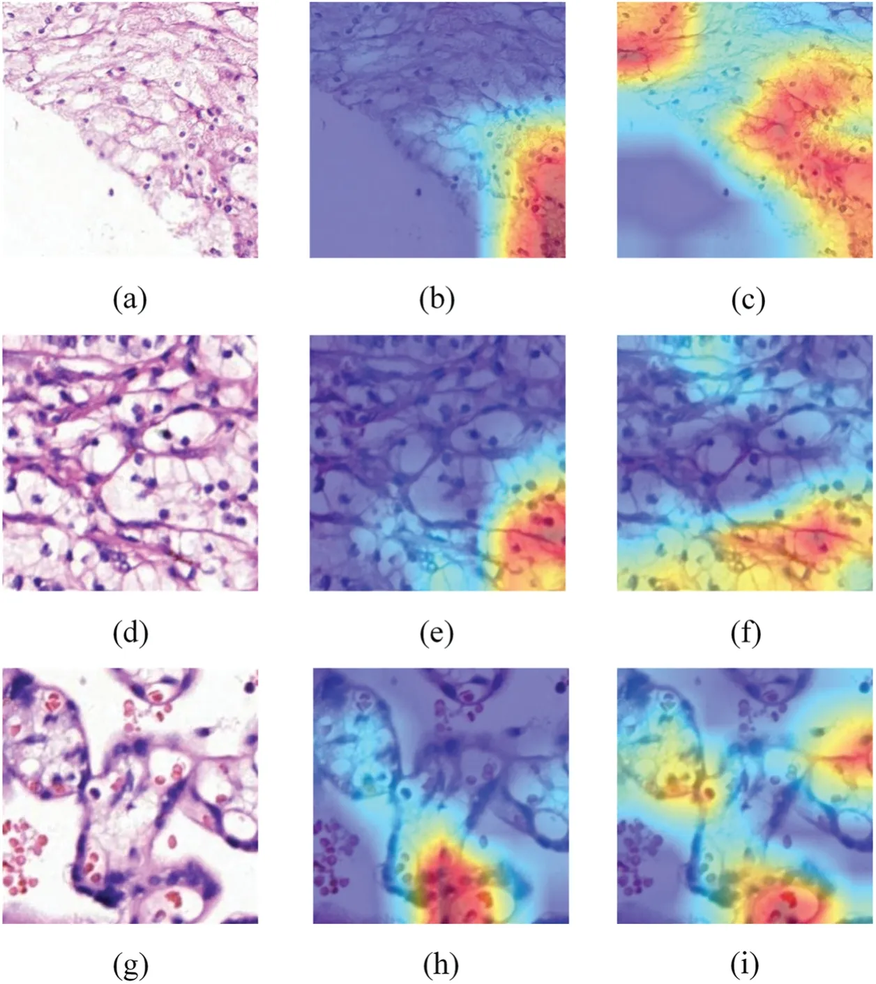
Figure 4: Exemplified class activation maps.(a,d,g): Raw pathology images;(b,e,h): Grad-CAM of ResNet50;(c,f,i): Grad-CAM of MsfNet.Red highlights the areas where the model focuses its attention on the prediction,while dark blue areas signify regions with low attention

In Fig.5,this study showed the t-SNE results of two methods: the left one uses raw test image data directly,while the other one uses features extracted from test image data by the MsfNet.t-SNE is a technique for visualizing high-dimensional data by reducing its dimensions,effectively revealing the structure and patterns within the dataset[39].As shown in Fig.5a,we consider the intensity values of each pixel as features of the data points and then the t-SNE algorithm was used to lower the dimensions of these high-dimensional features.The drawback of this approach is that the raw images contain a large amount of redundant information and noise,which can affect the results of the t-SNE plot,leading to a less clear distribution of data points in the low-dimensional space.Meanwhile,as shown in Fig.5b,we first employ MsfNet to extract features from the raw images,effectively capturing local features and global structural information within the images.After processing through the MsfNet,we obtain a set of more compact and expressive feature vectors.This study then applied the t-SNE algorithm to decrease the dimensions of these feature vectors,and the brown dotted curves were manually drawn onto the visualizations to mark the approximate border positions.Compared to using raw image data directly,this method exhibits a clearer distribution of data points in the t-SNE plot,better revealing the intrinsic structure and similarity within the dataset.

Figure 5:The t-SNE visualization results.(a)The t-SNE visualization of the raw dataset.(b)The t-SNE visualization of the features extracted by MsfNet

Therefore,according to the comparison of these two methods,the t-SNE plot after extracting features using MsfNet is more effective in revealing the structure and similarity information than directly applying t-SNE on raw image data.This is mainly because the MsfNet can efficiently extract key features from images,reducing the impact of noise and redundant information and resulting in a clearer distribution of data points in the t-SNE plot.

5.3 Comparative with Other Networks

In the testing phase,this study evaluated the performance of our proposed model,MsfNet,against several classic CNNs and vision transformer networks (ViT [40] and Swin-Transformer [41]).The performance metrics for these networks are presented in Tables 5 and 6.For a balanced comparison,all models were trained using the same dataset and evaluated under identical conditions.

In Table 5,the MsfNet outperforms all other networks with metrics of accuracy,precision,recall,and F1-score.This suggests that MsfNet is highly effective in comparison to the classic CNNs and vision transformer networks under the given experimental conditions.The superior performance of MsfNet may be attributed to its unique architecture and design choices,which contribute to more effective feature extraction and learning.Meanwhile,it can be seen from Table 6 that the AUC value of our proposed model in the ROC curve is only slightly lower than ResNet50(0.9957vs.0.9979)when identifying normal and performs better than other networks in identifying other categories.Generally,the proposed network outperforms other competitors under the AUC evaluation index.Subsequently,fusing the multi-scale feature map in the CNNs is a good trick to improve the performance of the network.However,it is worth noting that ViT and Swin-Transformer performed less effectively compared to other CNNs.This could be attributed to the fact that vision transformers rely more on large-scale training datasets and global semantic information,while CNNs excel at exploiting local critical details from the limited medical images available in this study.

Table 5: Comparison of the performance metrics(%)of different CNNs

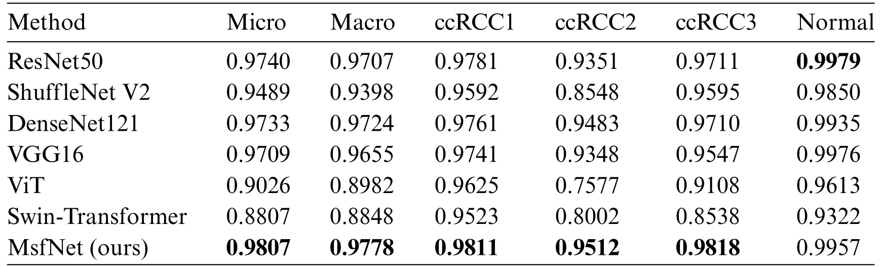
Table 6: Comparison of the AUC values of different CNNs

5.4 Comparative Analysis with Representative Studies

Finally,some representative studies on the assisted diagnosis of RCC in the past four years are summarized in Table 7.Among these eight studies,four focus on CT images,while the other four focus on histopathological images.These studies mainly employ radiomics and deep learning methods,aiming to predict ISUP grading and histological subtypes of RCC.As illustrated in Table 7,radiomics methods have achieved higher accuracy in predicting ISUP grading.The AUC values for[42–45]are 0.969,0.875,0.841,and 0.902(training set)/0.940(testing set),respectively.These results indicate that radiomics methods can distinguish ISUP grading of RCC patients with high sensitivity and specificity.

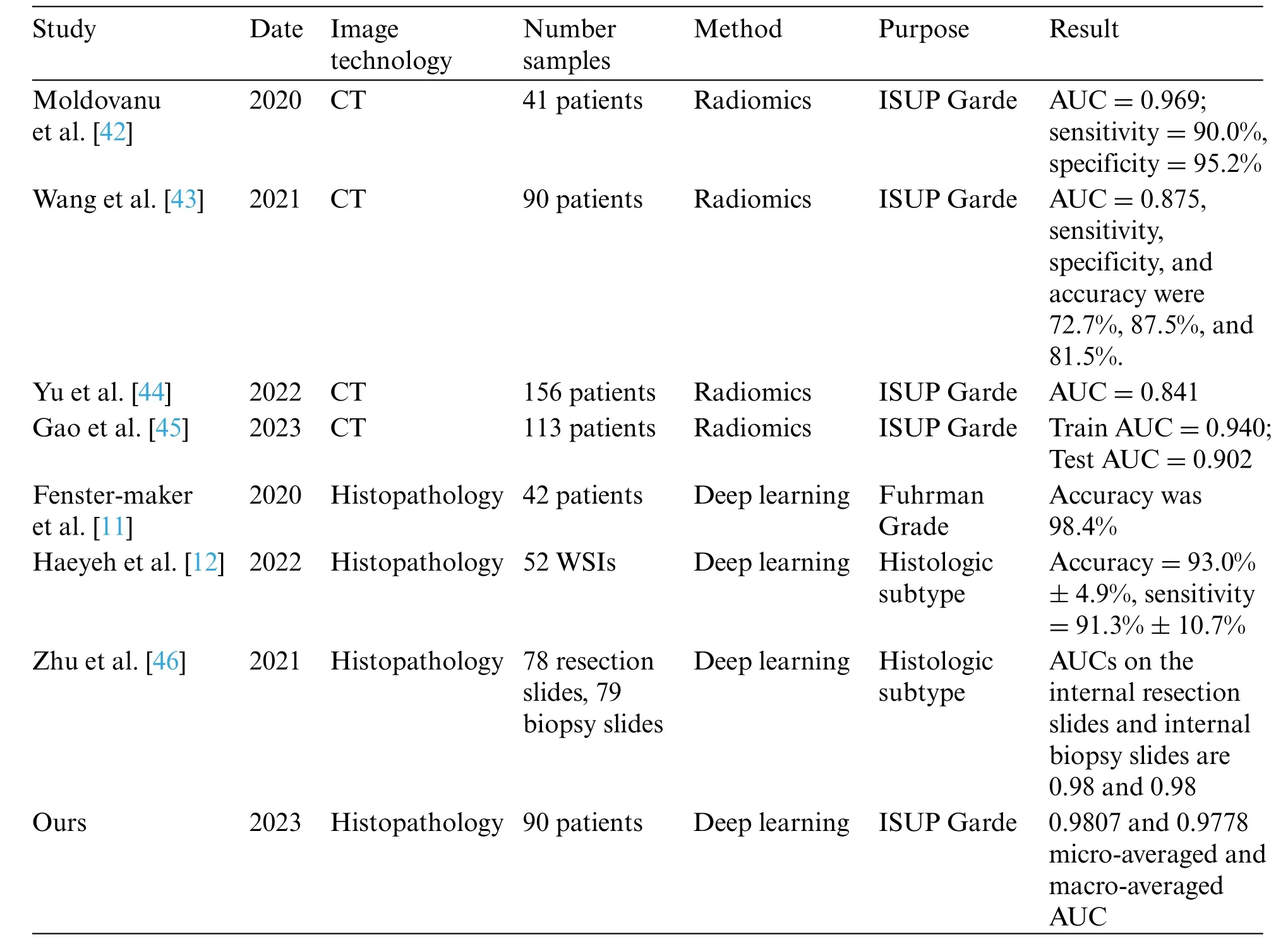
Table 7: Compare with the representative studies on the assisted diagnosis of RCC

At the same time,deep learning methods have obtained significant results in the analysis of histopathological images.The accuracy of reference [11],reference [12] and ours are 98.4%,93.0%,and 87.06%,respectively.Additionally,the AUC of reference[46]and ours are 0.98 and 0.9807(microaveraged)/0.9778 (macro-averaged),respectively.These achievements confirm the high accuracy and reliability of deep learning methods in predicting histological subtypes and ISUP grading of renal cell carcinoma.

Our study attains 0.9807 and 0.9778 micro-averaged and macro-averaged AUC.By employing deep learning models for ccRCC grading,our research addresses a gap in the field.The results demonstrate that our method exhibits high performance and accuracy in RCC auxiliary diagnosis,particularly in predicting ISUP grading of ccRCC using histopathology images.

In summary,significant progress has been made in RCC auxiliary diagnosis research in the past 4 years.Radiomics and deep learning methods have played important roles in improving the prediction accuracy of ISUP grading and histological subtypes for RCC patients.

6 Conclusion

In this study,a new deep framework MsfNet was introduced to predict the ISUP grade of ccRCC through the pathological image.This is achieved by fusing multi-scale information and reusing the shallow semantic information and the deep semantic information.We first trained the model on the training set divided by patients and tested the performance of the MSFNet on the testing set with independent patient data.The findings demonstrate that the proposed MSFNet can classify the ISUP grade of ccRCC with greater accuracy and better than other classification networks.In the future,we will further optimize our approach to enable prediction at the WSI level.Additionally,we plan to enhance the model’s capabilities by accurately identifying subtypes of RCC and achieving precise grading for different subtypes.Lastly,we envision the application of real-time computer-aided diagnosis in clinics,which can significantly save time for doctors and reduce missed detections.

Acknowledgement:Thanks for reviewers and editors for providing suggestions during review process.Funding Statement:This research was supported by the Scientific Research and Innovation Team of Hebei University(IT2023B07),the Natural Science Foundation of Hebei Province(F2023201069),the Postgraduate’s Innovation Fund Project of Hebei University(HBU2024BS021).

Author Contributions:The authors confirm contribution to the paper as follows: study conception and design: K.Yang,S.Chang,L.Xue;data collection: Y.Wang,M.Wang,H.Yang;analysis and interpretation of results:K.Yang,S.Chang,S.Liu;draft manuscript preparation:S.Chang,K.Liu,L.Xue.All authors reviewed the results and approved the final version of the manuscript.

Availability of Data and Materials:The data will be available on suitable request from corresponding author.

Conflicts of Interest:The authors declare that they have no conflicts of interest to report regarding the present study.