A Real-Time Small Target Vehicle Detection Algorithm with an Improved YOLOv5m Network Model

Yaoyao Du and Xiangkui Jiang

School of Automation,Xi’an University of Posts and Telecommunications,Xi’an,710121,China

ABSTRACT To address the challenges of high complexity,poor real-time performance,and low detection rates for small target vehicles in existing vehicle object detection algorithms,this paper proposes a real-time lightweight architecture based on You Only Look Once (YOLO) v5m.Firstly,a lightweight upsampling operator called Content-Aware Reassembly of Features (CARAFE) is introduced in the feature fusion layer of the network to maximize the extraction of deep-level features for small target vehicles,reducing the missed detection rate and false detection rate.Secondly,a new prediction layer for tiny targets is added,and the feature fusion network is redesigned to enhance the detection capability for small targets.Finally,this paper applies L1 regularization to train the improved network,followed by pruning and fine-tuning operations to remove redundant channels,reducing computational and parameter complexity and enhancing the detection efficiency of the network.Training is conducted on the VisDrone2019-DET dataset.The experimental results show that the proposed algorithm reduces parameters and computation by 63.8%and 65.8%,respectively.The average detection accuracy improves by 5.15%,and the detection speed reaches 47 images per second,satisfying real-time requirements.Compared with existing approaches,including YOLOv5m and classical vehicle detection algorithms,our method achieves higher accuracy and faster speed for real-time detection of small target vehicles in edge computing.

KEYWORDS Vehicle detection;YOLOv5m;small target;channel pruning;CARAFE

1 Introduction

Recently,urban traffic is increasingly being transformed into smart systems due to the accelerated development of smart city construction and the explosive growth of vehicle ownership.Object detection is essential in computer vision,and is a prerequisite technology for many practical problems,such as traffic scene analysis,intelligent driving,and security monitoring[1].Therefore,vehicle object detection is recognized as a key technology and core content in the research of intelligent vehicle systems and intelligent transportation systems,and it has significant research value and practical significance.

The development of Vehicle object detection has undergone two main stages: traditional algorithms and deep learning-based methods[2–4].Traditional vehicle detection algorithms mostly rely on sliding windows and manually designed complex feature representations to accomplish the detection task,but the performance of this method is often limited by the quality and quantity of the manually designed features.It is also computationally expensive and less robust in complex scenarios.In comparison,deep learning-based vehicle detection algorithms can achieve better performance in various computer vision problems by learning high-level feature representations.They have advantages like high accuracy,fast speed,and strong robustness in complex conditions.With the advancement of convolutional neural networks,the current trend in vehicle detection algorithms is to develop deeper and more complex networks to achieve higher accuracy.However,improving accuracy often comes at a cost.The existing vehicle detection algorithms exhibit high complexity,parameter count,and computational requirements,rendering them unsuitable for deployment on mobile and terminal devices with limited hardware resources.Moreover,real-world scenarios pose challenges for vehicle detection,including small-sized targets,high speed,complex scenes,limited extractable features,and significant scale variations.These issues render existing detection algorithms inadequate for detecting small vehicle targets.Therefore,the purpose of this study is to propose an optimized model for vehicle detection,specifically addressing the shortcomings of previous studies,such as high detection costs,poor detection rates,and inaccurate detection of small-sized vehicle targets[5,6],based on analyzing and comparing existing deep learning object detection models.

The organization of the remaining files is as shown below.In Section 2,this paper introduced some related research on vehicle object detection.Section 3 provides the benchmark detection model this article selected.Section 4 describes the specific improvement plan in detail.The detailed experimental settings,experimental results,experimental analysis,and comparison with other models are presented in Section 5.The final section presents the conclusion.

2 Related Works

Currently,vehicle object detection algorithms based on deep learning can be grouped into two types based on their detection methods.The first type is the two-stage detection algorithm using candidate boxes,with RCNN as its typical representative [7].It predicts the final target box by generating a set of candidate boxes,and then classifying and regressing these boxes.The second type is the one-stage detection algorithm using regression,with YOLO as its typical representative[8–11].It directly convolves and pools the image to generate candidate boxes,and performs classification and regression at the same time to detect the vehicle object.The two-stage detection algorithm is more accurate but poorer detection speed and higher computational complexity.In contrast,the one-stage detection algorithm focuses more on the balance between detection speed and accuracy.It is widely used for vehicle detection.

Yang et al.[12] proposed an improved vehicle detection system that combines the YOLOv2 detection algorithm with the long short-term memory(LSTM)model.Initially,all vehicle categories were amalgamated and low-level features were removed.The detected targets were then enhanced by a dual-layer LSTM model (dLSTM) to improve the accuracy of detecting vehicle objects.However,the improved model is somewhat unwieldy and does not effectively reduce computational load.Stuparu et al.[13] proposed a high-performance single-stage vehicle detection model based on the RetinaNet architecture and the Cars Overhead With Context dataset(COWC).The model is accuracy improved to 0.7232,and the detection time is approximately 300 ms.Zhang et al.[14] proposed a vehicle detection network(SGMFNet)using self-attention.This network is enhanced by adding the Global-Local Feature Guidance (GLFG) module,Parallel Sample Feature Fusion (PSFF) module,and Inverted-residual Feature Enhancement(IFE)module to improve the feature extraction capability and multi-scale feature fusion effect of small vehicle targets.However,the network is too large to be deployed on embedded devices.Zhao et al.[15] proposed an attention-based inverted residual block structure called ESGBlock to replace the original backbone network in YOLOv5 detection algorithm.This method effectively reduces parameters and computation.The GSConv module is introduced in the feature fusion layer with knowledge distillation to address the problem of highdimensional feature information loss and complexity.Although the improved algorithm is more in line with the requirements of lightweight deployment on embedded devices,it sacrifices part of the detection accuracy and does not improve detection of small objects.Mao et al.[16] introduced the Spatial Pyramid Pooling (SPP) module based on the YOLOv3 detection algorithm,and combined it with Soft Non-Maximum Suppression(Soft-NMS)and the inverted residual technology to detect small and occluded vehicles better.However,the network structure of the model is too complex,which makes training difficult.Cheng et al.[17]optimized the YOLOv4 detection algorithm by introducing lightweight backbone networks such as MobileNetV3,as well as the Multiscale-PANet and soft-merge modules,which improved the mAP index to 90.62%while achieving 54 FPS and 11.54 M parameters.These optimization measures have simplified the model and accelerated the detection speed.However,the model’s detection accuracy did not improve significantly.Liu et al.[18] proposed a lightweight feature extraction network,Light CarNet,based on the YOLOv4 detection algorithm.According to the characteristics of detecting vehicle targets at different scales,a four-scale feature bidirectional weighted fusion module was designed for classification and regression.The experiments demonstrated a 1.14%increase in mAP value and improved detection of small vehicle targets while maintaining realtime detection.However,this method also increased the complexity and number of parameters of the model.

The above-mentioned method has contributed to vehicle target detection,but three important issues still need to be urgently addressed.

(1)Detection of vehicles with small targets and fuzzy targets is poor.

(2) Faced with complex network structures,the models need a lot of computing resources and costly model training.

(3)In practical applications,it is essential to not only meet the requirement for high accuracy but also consider real-time performance.

To address the above-mentioned issues,this paper proposes a real-time and efficient small target vehicle detection algorithm based on the YOLOv5m detection algorithm,with lightweight improvements to enhance the detection ability for small target vehicles.In conclusion,the following are the contributions made by this paper.

(1)To enhance the model’s utilization of deep semantic information,this paper proposes the use of a lightweight upsampling operator instead of the traditional nearest-neighbor interpolation operator.By reorganizing contextual features,it effectively improves the detection of vehicle objects in complex scenes.

(2)To improve the detection of small target vehicles,this paper introduces a dedicated small target prediction layer within the model’s output prediction layers.This enhances the model’s focus on small target vehicles.

(3)This paper proposes an enhanced FPN+PANet architecture to improve the fusion capability of the model for small target vehicle features.

(4) Based on the contribution of model channels to model performance,this paper applies channel pruning and compression operations to the improved YOLOv5m network model.It removes redundant channels,thereby reducing model complexity while further improving network detection performance.

3 YOLOv5m Algorithm

The YOLO series of network models has become one of the top-performing models in object detection due to its balance of speed and accuracy.YOLOv5 is the fifth generation of the YOLO series algorithm[19–21],proposed by Ultralytics in May 2020.There are five pre-trained models of YOLOv5,which differ by the width and depth parameters and are named YOLOv5n,YOLOv5s,YOLOv5m,YOLOv5l,and YOLOv5x.Table 1 shows the width and depth parameters and the corresponding model sizes for each pre-trained model.

Table 1: Summary of the network model parameters for the YOLOv5 algorithm

Among the five pre-trained models,as the model size and detection accuracy increase,the detection rate decreases.Therefore,taking into account detection rate,accuracy,and model size,this research selects the YOLOv5m-6.0 architecture as the basis for optimizing and improving the small target vehicle detection algorithm.Fig.1 depicts the network structure of YOLOv5m-6.0,which comprises four main parts:input,backbone,neck,and prediction.The training images have a size of 640 pixels by 640 pixels and consist of three color channels.

The input network applies mosaic data enhancement to the input vehicle image by simultaneously reading in four images and randomly scaling,cropping,and arranging them before stitching them together.By incorporating information from these diverse images,the model’s dataset is enriched,improving its robust performance and enhancing small target vehicle detection in this paper.Moreover,the network employs adaptive anchor box calculation methods to set the optimal initial anchor boxes,facilitating iterative optimization of network parameters during training.Additionally,the original image is preprocessed to a size of 640×640×3 using adaptive image scaling,which reduces redundant information and improves model inference speed compared to traditional resize operations.

The backbone network of YOLOv5m-6.0 has three primary components: the CBS (kernel size(k)=6,stride (s)=2,padding (p)=2) module,CSPDarkNet53,and the Spatial Pyramid Pooling Fast (SPPF) module.In this context,k=6 represents a convolution kernel size of 6 × 6,s=2 indicates that the kernel slides 2 pixels at a time,and p=2 signifies zero-padding of 2 pixels around the input image.Compared to the old version,YOLOv5m-6.0 replaces the focus module for ease of model export and employs multiple small pooling kernels in the SPPF module,rather than a single large kernel in the SPP module.This enhances the network’s ability to recognize fuzzy small targets in complex backgrounds while also improving its computational speed.Furthermore,YOLOv5m-6.0 uses Leaky Rectified Linear Unit(Leaky ReLU)as the activation function,with its calculation formula and derivatives shown in Eqs.(1)and(2).

whereαis generally set to 0.01,and its corresponding function and derivative function curves are shown in Fig.2.

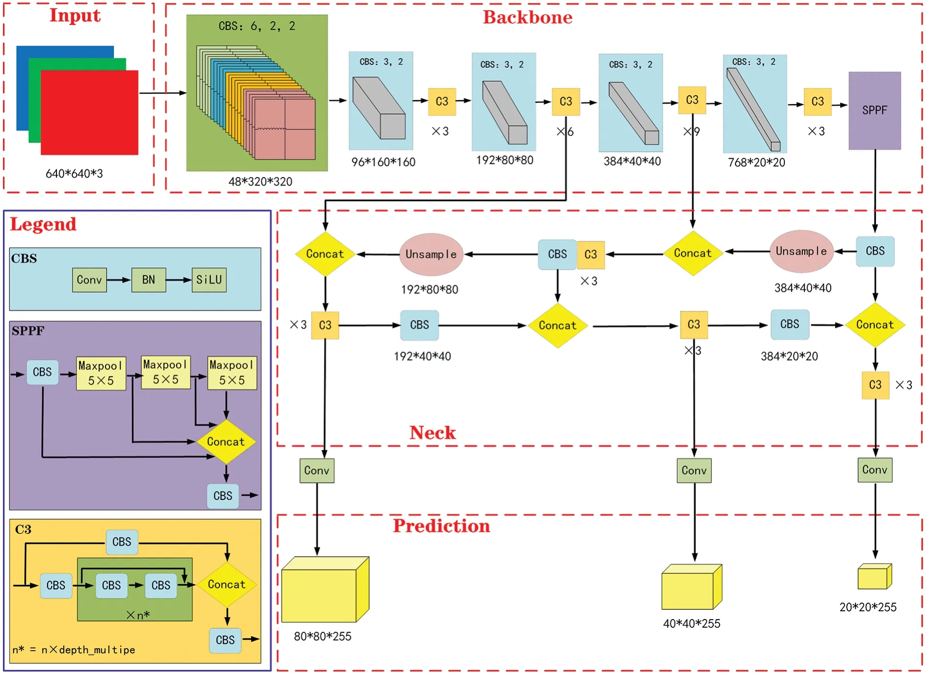
Figure 1:YOLOv5m-6.0 algorithm network model structure

Since it is a segmented function,it cannot maintain the same relational prediction for positive and negative input values,resulting in unstable performance results,and there are also intermittent points in the derivative function.

Therefore,YOLOv5m-6.0 uses the Sigmoid Weighted Linear Unit (SiLU) instead of the old version of Leaky ReLU as the new activation function.Its calculation formula and derivatives are given by Eqs.(3)and(4),and their corresponding function and derivative function curves are shown in Fig.3.

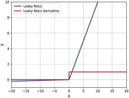
Figure 2:Leaky ReLU activation function and its derivatives

Figure 3:SiLU activation function and its derivatives

The SiLU activation function is more suitable for depth models because it is derivable everywhere and its derivative function satisfies the properties of continuity,smoothness,nonmonotonicity,and constant greater than 0.

The neck network resides between the backbone network and the prediction network,consisting of the Feature Pyramid Network (FPN) and the Path Aggregation Network (PANet).As shown in Fig.4,where FPN is the top-down propagation path [22].Firstly,a 2-fold upsampling operation is performed on the small-sized feature map.Secondly,a splicing fusion operation is performed on laterally connected same-sized feature maps.Then the fused feature maps undergo a 3×3 convolution operation to remove the blending effect caused by upsampling.Repeat the operation stage by stage,thus transmitting the deep strong semantic information to the shallow layer.And PANet is the bottomup propagation path[23].Firstly,the large-sized feature map is downsampled 2-fold.Then the feature maps of the same size connected with the lateral ones through splicing fusion and convolution.Repeat the operation stage by stage,thus transferring the strong localization information from the shallow layer to the deep layer and further enhancing the network is ability to extract fusion features.The structure enhances the model’s ability to detect targets of different scales,increases feature diversity,and improves overall robustness.

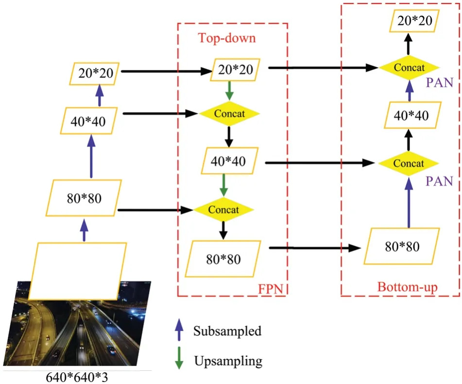
Figure 4:FPN and PANet structure

As the output end,the prediction network is used to predict and return the target.YOLOv5m-6.0 contains three prediction layers with dimensions of(80 ∗80 ∗255),(40 ∗40 ∗255),and(20 ∗20 ∗255),which are used to detect large,medium,and small-scale targets respectively.CIOU_LOSS is used as the loss function of the prediction frame of the network during training as shown in Eq.(5).It considers three important geometric factors,which are overlapping area,centroid spacing ratio,and centroid aspect ratio.Compared with the old version,the speed and precision of the prediction frame regression have been improved effectively.

The termα×Vin the equation uses the bounding box aspect ratio scale information,αis a positive balance parameter,andVis a measure of the consistency of the aspect ratio.It is calculated as follows:

The equation uses the intersection over union(IOU)metric to account for the overlapping area factor,which is calculated as follows:

In the equation,B=(x,y,w,h)andBgt=(xgt,ygt,wgt,hgt)represent the position parameters contained in the predicted frame and the marked frame,respectively.

To filter the predicted frames,the algorithm uses a weighted Non-Maximum Suppression(NMS)approach which enables the detection of overlapping targets without requiring additional computational resources.

Based on the YOLOv5m-6.0 network architecture,it can be observed that the neck feature fusion network layer,due to the use of nearest-neighbor upsampling,neglects the semantic information of the extracted vehicle object features,leading to a decrease in the effectiveness of vehicle object detection.Therefore,it is necessary to replace the upsampling module to enhance the utilization of vehicle features and redesign an enhanced feature fusion network structure to improve the fusion capability for small-sized vehicle features.Furthermore,since the output only includes prediction layers of three scales,the feature extraction performance is poor when detecting vehicle objects with smaller proportions.Hence,it is crucial to design corresponding anchor boxes for small-sized vehicle objects to enhance their attention.Additionally,the overall network structure contains a large number of parameters and computational complexity,necessitating lightweight model compression operations.

4 Methodologies

This section primarily introduces components used to enhance the detection performance of small target vehicles,including the lightweight upsampling operator CARAFE,small target prediction layers,and the channel pruning compression process proposed in this paper.Additionally,a detailed diagram of the improved network model structure is provided.

4.1 Lightweight Upsampling Operator CARAFE

The YOLOv5m network utilizes the nearest neighbor interpolation algorithm to upsample feature maps,as illustrated in Fig.5.This algorithm maintains pixel values of the transformed pixels to be the same as those of the nearest input pixel.Eqs.(9)and(10)define the calculations involved,where(srcX,srcY)represents the original image’s pixel coordinates,and(dstX,dstY)represents the sampled image’s pixel coordinates.The termssrcWidth,srcHeight,dstWidth,anddstHeightsignify the dimensions of the original and sampled images,and the functionround(x)rounds x to the nearest integer using the principle of rounding half up.Consequently,the sampled pixel values(dstX,dstY)are equivalent to the original image’s calculated pixel values(srcX,srcY).

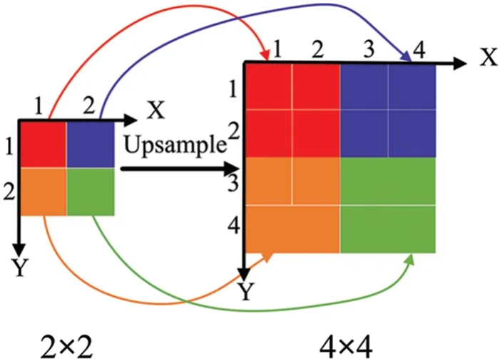
Figure 5:Neighbor interpolation algorithm

Therefore,the nearest neighbor interpolation algorithm solely relies on the spatial proximity of pixel points to establish the upsampling kernel.It fails to leverage the abundant semantic information within the feature map.Moreover,its perceptual field of vision is very small,only 1×1 in size,thus it underutilizes the surrounding information.

To improve the utilization of feature semantic information while controlling both the number of parameters and computational complexity,this paper introduces a lightweight upsampling operator called Content-Aware Reassembly of Features(CARAFE)to improve the network.Assuming input size isH×W×Cand upsampling rate isσCARAFE generates a new feature map of sizeσH×σW×C.The structure of the CARAFE network is shown in Fig.6.

CARAFE consists of two key modules [24–28]: the kernel prediction module and the contentaware reassembly module.It can utilize rich contextual information from lower levels to predict the reassembled kernels and reorganize features within the predetermined neighborhood.Assuming that the upsampling kernel size isKup×Kup,the procedure is as follows:

(1)Kernel prediction module

The module generates reconfigured kernels in a content-aware manner via three sub-modules:channel compressors,content compressors,and kernel normalizer.

Firstly,to reduce the number of parameters and computation,the input feature mapFis passed through a channel compressor composed of 1×1 convolutional layers so that the number of input feature channels is compressed fromCtoCm.Secondly,the compressed feature map is fed to the content encoder,and a 3 × 3 convolution is used to generate a reconstructed kernel with the size ofH×W×(σ2×,and perform a sub-pixelShuffle scaling operation on it to resize it to sizeσH×σW×[29].Finally,to ensure that the distribution of input features remains unchanged,eachKup×Kupreassembly kernel is normalized along the channel dimension using the softmax function,ensuring that the weights of each reassembly kernel sum up to 1.

(2)Content-aware reassembly module

The module utilizes the generated reassembly kernels to reassemble the features,outputs a new feature mapF′that contains semantic information.

Firstly,the (x,y) coordinates on the output feature mapF′are correspondingly mapped to(x′,y′) on the input feature mapF.The mapping relationship is shown in Eq.(11).Secondly,the reshaping operation is performed on the recombined kernel at the corresponding position to generate a perceptual field with the size ofKup×Kup.Then,the inner product is performed with the neighborhood centered at (x′,y′) on theF.It is worth noting that the same reshaping kernel is shared at the same position.Finally,theF′with the sizeσH×σW×Cis output.

The ⎿」 in the equation represents the floor function,which rounds down to the nearest integer.The calculation of the lightweight upsampling operator CARAFE is shown in Eq.(12).

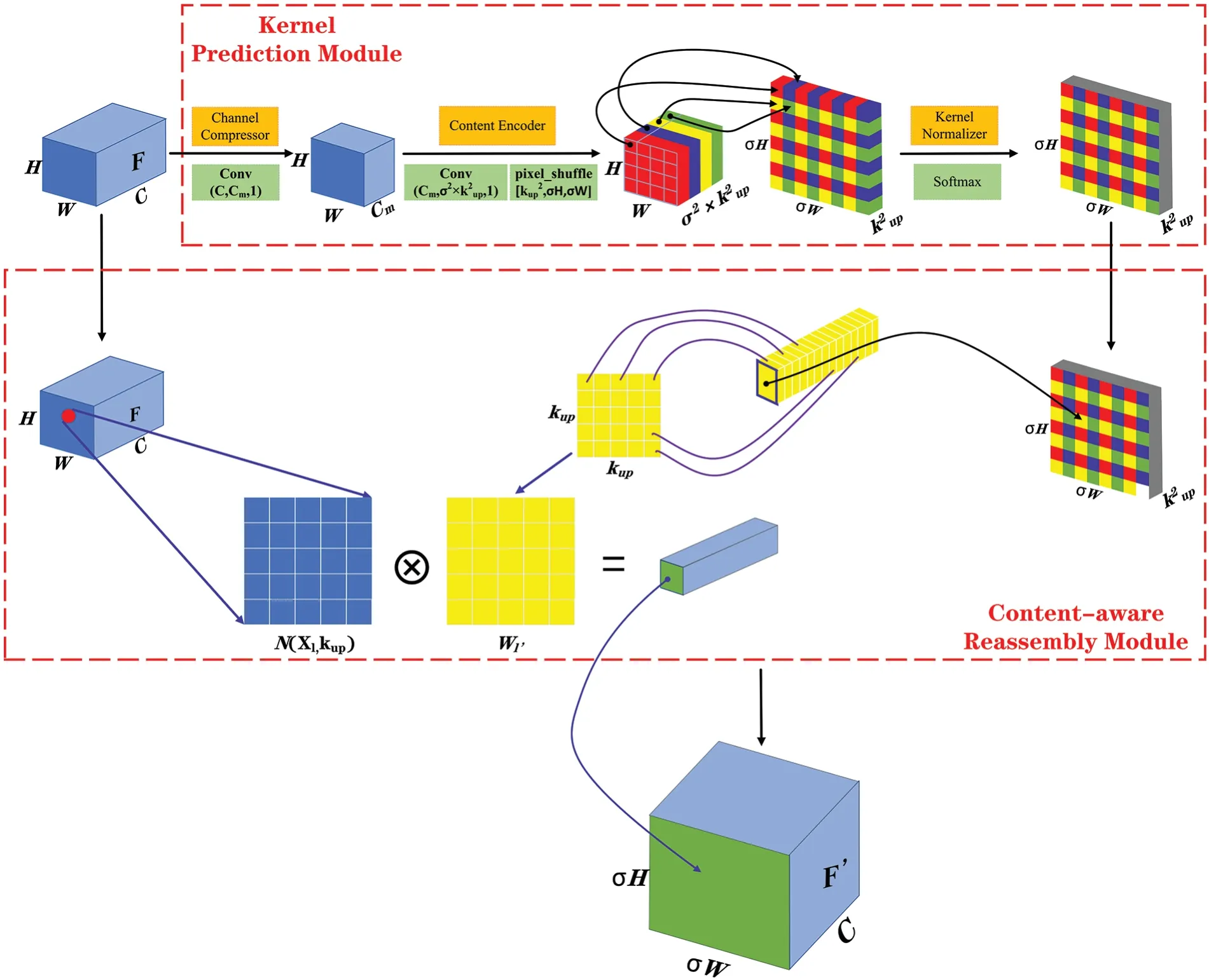
Figure 6:The overall framework of CARAFE

4.2 Adding Tiny Target Prediction Layers

The YOLOv5m network model before improvement struggles to capture feature information from small-scale vehicles,impeding learning performance,which makes the detection of small target vehicles have seriously missed detection and false detection in practice.There are three main reasons:

(1)The network subsampling multiplier is very large,so small target vehicles can not occupy pixels.

(2)The network perception field is large,which makes the perceived small object features contain a large number of surrounding worthless features.

(3)The deep and shallow feature maps in the network are not well-balanced in semantic and spatial attributes.

Therefore,to enhance the attention of the network to small target vehicles and improve the detection performance,it is proposed to add a tiny target prediction layer with a perceptual field of 4×4 size based on the three target prediction layers of large[30–33],medium and small of the original network.The corresponding feature fusion network has been redesigned.The improved network with the prediction frame size settings in each feature layer is presented in Table 2.Fig.7 shows the structure of the improved FPN+PANet.

Figure 7:Improved FPN+PANet structure

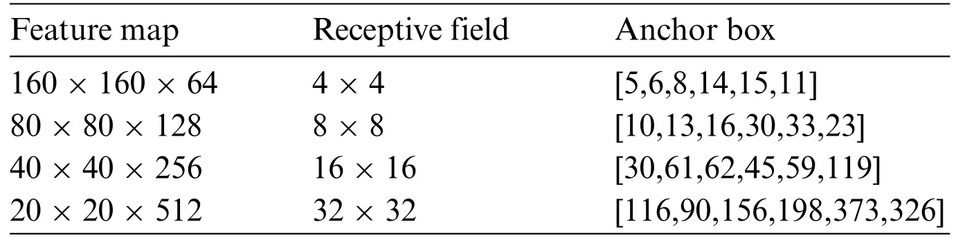
Table 2: Detect feature map information

4.3 Channel Pruning Compression

This paper uses the improved YOLOv5m network as the input model and apply channel pruning and compression operations to reduce computational complexity [34–37],improve generalization performance,and enhance the network’s accuracy on low-resource devices.Specifically,this article integrates sparse regularization training to identify and prune the low-performance channels,followed by fine-tuning to further improve accuracy.Fig.8 illustrates the implementation flow of our channel pruning and compression methodology.

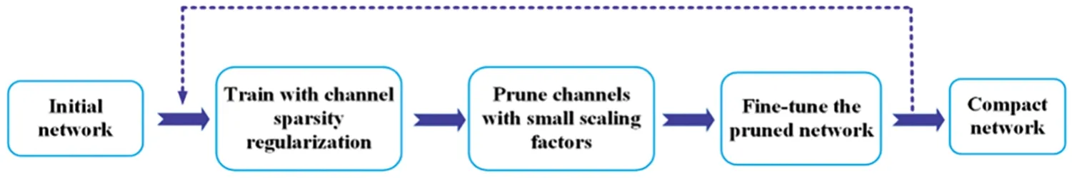
Figure 8:Channel pruning and compression flow chart

Step1:Sparse Regularization Training

In modern neural networks,it is common to use Batch Normalization(BN)layers after convolutional layers.The data output by the convolution layer is distributed within a reasonable range through translation and scaling,to speed up the training and convergence of the network and improve the generalization performance.LetZinandZoutbe the input and output of the BN layer,respectively.AndμBandσBrepresent the mean and standard deviation of the input samples within a batch.Then the BN layer is calculated as shown in Eqs.(13)and(14).

The BN layer uses learnable scaling factorsγand translation parametersβto normalize the input values.However,to prevent the possibility of division by zero,a small constantεis added to the denominator.When the scaling factorγtends towards zero,the output of the convolutional module becomes independent of the input.In such cases,the channel can be considered less important for model performance,and the weight ofγserves as an indicator of channel importance for potential pruning.Therefore,γcan be used as an indicator to identify low-performance channels effectively.

Therefore,by sparse regularization of the scale factorγin the BN layer and joint training of the network weights,theγin the BN layer in the neural network converges to 0,and a sparse network with friendly pruning is obtained.The loss function of sparse training is shown in Eq.(15):

The above equation consists of the sum of two terms.The first term is the loss function of the original YOLOv5m algorithm,where(x,y)represents the training input and label values,Wdenotes the network trainable weight parameter,and the second term is the loss function of the sparse training scale factorγ,whereλis the sparsity rate,the larger the value,the greater the sparsity of the network,and also has a greater impact on the network accuracy,which is used to balance the loss of the front and back two terms.In the second term,‖γ‖1is the L1 regularization term for the scaling factor.It is used to drive the scaling factorγtowards 0,thus achieving network sparsity.The calculation of this term is shown in Eq.(16),whereΓrepresents the set of all scaling factors in the network.

Step2:Pruning Operation

After the network is trained by sparse regularization,the scaling factorγcorresponding to the majority of channels will tend to be 0,which means that the contribution of these channels to the network performance is very low.Therefore,this paper sorts all the scaling factorsγ,then set the pruning rate and adopt a specific pruning strategy,and finally prune all the inputs and outputs of the channels below the threshold value,to get a more lightweight compression model.

The channel pruning schematic is shown in Fig.9.The left image represents a sparse network,while the right image represents a compressed network after pruning.By performing channel pruning operations,the channelsCi2andCi4in the left image,where the scaling factors tend towards 0,are eliminated.Finally,the remaining channels are reorganized to obtain a pruned and compact network.

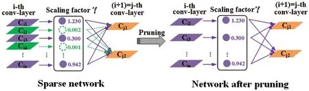
Figure 9:Schematic diagram of channel pruning

According to the characteristics of the small target vehicle detection network,a global threshold strategy is adopted to prune,that is,whether to prune the channel or not is decided by introducing the global threshold.Firstly,the scaling factorγof all channels in the sparse network is sorted,and then the lower scaling factorγis selected as the global thresholdaccording to the predetermined pruning rate,and the channels below this threshold in the network are eliminated.In addition,the single threshold control pruning can cause all channels in a layer of the network to be pruned,thus destroying the regular structure of the original network.Therefore,it is necessary to introduce a local safety thresholdτagain,that is,to eliminate channels that are less than the global thresholdand the local thresholdτlayer by layer to prevent excessive pruning.

After pruning,the number of parameters in the network model is significantly reduced,resulting in a more compact model.However,when targeting fine-grained target detection tasks,increasing the pruning rate may lead to a slight decline in precision.To address this issue,it is necessary to fine-tune the pruned model and use the fine-tuned model as the final compressed model.

The pruning algorithm can be classified into two categories based on the pruning operation process:iterative and one-shot.

Iteration: Pruning is carried out layer by layer,and it needs to be retrained and fine-tuned after each pruning.However,since this method requires multiple iterations and the consumption of computational resources increases with the complexity of the network structure.It is not used.

One-shot:After sorting the scale factorγ,the BN layers in the network are pruned simultaneously to remove the redundant parameters and then retrained.Not only does it reduce the consumption of computational resources,but it also significantly improves the detection accuracy.Therefore,this paper adopts a one-shot approach to prune the model.

4.4 Improved Network Structure Diagram

This paper presents the improved model structure of the YOLOv5m-6.0 algorithm,as shown in Fig.10.While retaining the original backbone feature extraction network,this paper replaces CARAFE with a new upsampling method and add small target prediction layers.This paper also redesigns the enhanced feature fusion network.Finally,this paper applies channel pruning to the model structure and use the compressed model as the final improved model.

Figure 10:Improved YOLOv5m-6.0 network model structure diagram

5 Experiments

This section aims to verify the effectiveness and rationality of the improved YOLOv5m algorithm in small target vehicle detection.To achieve this,this article will introduce the dataset used for model training,the experimental platform environment,relevant hyperparameters,evaluation metrics,analyze the results,and show the detection comparison effect.

5.1 Build the Dataset

To test the method’s feasibility and effectiveness,this study uses the VisDrone2019-DET large public dataset to train and evaluate the model.The dataset,developed by the AISKYEYE team at Tianjin university’s machine learning and data mining laboratory,is an open-source dataset for UAV high-altitude scenes that includes 10 categories of interest,such as cars,people,vans,and others.This experiment focuses on car detection,and filtering techniques were applied to extract a representative and diverse sample set of 8178 images for training and detection.Of these,90%were used to create the training set consisting of 7275 images,while the remaining 10%were allocated to the test set containing 903 images.The dataset covers various traffic scenarios,including streets,highways,and intersections,and diverse challenging environmental backgrounds,such as strong light,low light,rainy weather,and foggy conditions,reflecting typical and relevant real-world conditions.Fig.11 shows the distribution of sample label scales in the training set,where the width and height of the label frame are respectively represented by the horizontal and vertical axes.The distribution of data points indicates the dataset contains a large number of small-scale target vehicles that meet the requirements of the experimental training.

Figure 11:Schematic diagram of the label scale of the training set sample

5.2 Experimental Environment

The experiment used PyTorch on Windows 10.A virtual environment was created using Anaconda Navigator with Python 3.9,PyTorch 1.10,TensorFlow 2.7.0,and Cuda 11.2 installed.The hardware configuration included a 6X65-2680 V4 CPU and NVIDIA RTX4000 GPU.The iterative training utilized a modified YOLOv5m network structure and included an initial learning rate of 0.01,batch size of 16,65%pruning rate,0.0002 sparse rate,and 100 epochs.

5.3 Model Performance Evaluation Metrics

To accurately evaluate the improved YOLOv5m for detecting small target vehicles on the VisDrone2019-DET dataset,this paper analyzes its lightweight and detection performance using various metrics.These metrics include the number of parameters,recall,average precision when the threshold IOU is 0.5(mAP@0.5),average precision over IOU thresholds ranging from 0.5 to 0.95 in increments of 0.05 (mAP@0.5:0.95) [38],Giga FLoating-point Operations Per Second (GFLOPS),Frames Per Second(FPS),and Model Size.These metrics provide a comprehensive measurement of the model’s performance from various aspects and perspectives.The calculation formula is as follows:

In the above formula,three dichotomous parameters are selected which are defined in Table 3.Where 1 and 0 indicate whether the result is a vehicle or not,respectively.True Positives(TP)represents the number of correctly detected vehicle samples.It refers to the samples where both the ground truth and the model prediction indicate the presence of vehicles.False Positives(FP)represents the number of falsely detected vehicle samples.It refers to the samples where the ground truth indicates the absence of vehicles,but the model incorrectly predicts them as vehicles.False Negatives (FN) represents the number of missed vehicle samples.It refers to the samples where the ground truth indicates the presence of vehicles,but the model incorrectly predicts them as non-vehicles.Average Precision(AP)represents the area under the precision-recall curve.The value of AP is calculated for each class,and n represents the total number of classes.HW indicates the output feature map size.K denotes the convolutional kernel size,CinandCoutrepresent the input and output channel counts,respectively.FPS is the images detected per second,and t represents the time consumed for detecting a single image.

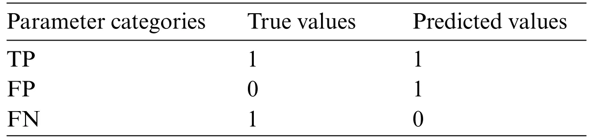
Table 3: Definition of second classification parameters

5.4 Experimental Results and Analysis

This section provides a detailed introduction to the experimental training results of the improved algorithm from the perspectives of lightweight performance and testing performance,and analyzes and verifies them.Finally,a comparison of the detection performance with the current mainstream vehicle detection algorithm models is conducted under the same experimental environment and parameters.

5.4.1 Sparse Regularization Training

As the selection of the sparsity rate directly influences the level of network sparsity,which in turn affects the effectiveness of subsequent model compression and detection performance,this paper assesses the network sparsity level across various sparsity rates.The optimal value of the sparsity rateλis then chosen based on the application requirements.Fig.12 illustrates the distribution of the scaling factorγin the BN layer of the improved network model after 100 rounds of iterative training using different sparsity ratesλduring sparse regularization training.

Figure 12:Schematic diagram of the variation of the scaling factor for different sparsity rates

When the sparsity rateλis set to 0,indicating the absence of sparsity training,the scaling factorsγin each layer follow a normal distribution.As the number of training round increases,theγvalues remain mostly unchanged and centered around 1.0.Consequently,the model cannot be compressed at this stage.

When the sparsity rateλ=0.0001,as the network training progresses,theγvalues of each layer gradually approach 0,and the network gradually becomes sparse.After training,theγvalues of each layer are concentrated around 0.73.Consequently,the model can be compressed to a certain extent.

When the sparsity rateλ=0.0002,the speed of network sparsification increases,and finally,it is concentrated around 0.49.Consequently,the model can be significantly compressed.

When the sparsity rate λ increases to 0.0003,the degree of network sparsity increases significantly.After training,the γ values of each layer are concentrated around 0.25.Consequently,the model can be compressed to an extremely high degree.

Table 4 presents the average detection precision of the sparse-trained models at various sparsity rates.The results indicate that for sparsity rates of 0,0.0001,and 0.0002,the average detection precision remains relatively stable as the network sparsity increases.However,a noticeable decline in the average detection precision occurs when the sparsity rate reaches 0.0003.

Table 4: The average detection precision of the sparse-trained models under different sparsity rates

Based on the aforementioned experiments,it was observed that a sparsity rate of λ=0.0001 results in relatively low model sparsity and inadequate compression effect.Conversely,a sparsity rate of λ=0.0003 leads to excessive model sparsity and significant precision loss.Thus,to ensure a balance between compression effect and detection performance,the optimal sparsity rate of λ=0.0002 is selected.

5.4.2 Channel Pruning

After completing sparse regularization training,the selection of the channel pruning rate becomes crucial.If a channel pruning rate is chosen too small,the model’s lightweight effect may be compromised.Conversely,selecting a channel pruning rate that is too large can potentially have destructive effects on the model.Hence,this paper pruned the model using various channel pruning rates and analyzed the average detection precision of the pruned model,as depicted in Fig.13.The horizontal axis represents the pruning rate,while the vertical axis represents the corresponding average detection precision value.From the figure,it is evident that the model’s evaluation detection precision remains stable when the pruning rate is below 65%.However,there is a rapid decline in the average detection precision when the pruning rate exceeds 65%.To strike a balance between the network’s detection precision and lightweight requirements,the experiment ultimately determined the channel pruning rate as 65%.

Figure 13:The impact of different pruning rates on model accuracy

The statistics of the number of output channels for each layer of the network before and after pruning are shown in Fig.14.The red bar chart represents the number of output channels in each layer of the network before channel pruning,totaling 19,600.The blue bar chart represents the number of output channels in each layer of the network after channel pruning,totaling 10,560.From the figure,it can be observed that a total of 9,040 redundant channels were pruned in all layers of the model,indicating a significant reduction in redundant channels and effective compression of the model.

Fig.15 shows a comparison of the parameter quantity,calculation quantity,and model size before and after pruning in a columnar diagram.The red bar represents the values before channel pruning,while the green bar represents the values after channel pruning.It can be observed from the figure that after pruning,the number of parameters in the model decreased to 35.26%of the original value,with a reduction of 64.74%in redundant parameters.The GFLOPS also decreased by 72.18%,and the size of the pruned model was reduced by 63.25%compared to the original model.Further validation confirmed that the channel pruning method used in this study effectively compressed the YOLOv5m network model and saved network resources.

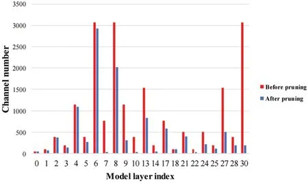
Figure 14:Comparison of channel number before and after pruning

Figure 15:Lightweight comparison of models before and after pruning

5.4.3 Comparative Analysis of Experiments

To validate the feasibility and robustness of the proposed improvement scheme,three groups of controlled experiments were conducted for analysis,as shown below:

• This paper conducted ablative experiments comparing the original YOLOv5m network model(Model A)with Model B,Model C,and Model D.Model B replaced the upsampling operator with a lightweight bottle operator,while Model C added a small target prediction head on top of the original model.Model D combined the improvement methods of both Model B and Model C.

• The original network Model A is compared and analyzed with the final improved Model E.

• This paper compared and analyzed the experimental results of Model E with those of other classic mainstream vehicle detection algorithms,in order to assess the effectiveness Model E.

Table 5 presents a comparison of lightweight metrics parameters for each model.Meanwhile,Table 6 includes the experimental results for each model’s training,and a comparison of parameters for detecting performance indexes.

Table 5: Lightweight data comparison

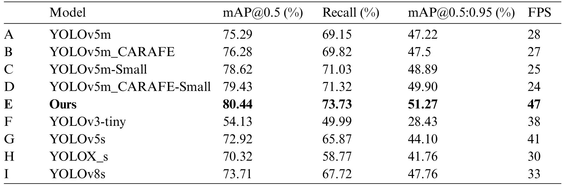
Table 6: Testing performance data comparison

Fig.16 displays graphs of the network’s average accuracy,loss function,and recall variation during training.The horizontal axis showing iterations,while the vertical axis showing the corresponding values of mAP@0.5,loss function,and network recall rate.The green line in the figure represents the experimental result curve of the final improved model.From the figure,it can be observed that the improved algorithm achieves higher detection accuracy and recall rate compared to other detection models.Additionally,it demonstrates faster convergence,further validating the effectiveness of the improvement method.

The experimental results of Model A and Model B in Tables 4 and 5 show that replacing the lightweight upsampling module CARAFE has slightly increased the algorithm’s parameter and computational complexity.However,the average detection accuracy and recall rate have improved by 0.99% and 0.67%,respectively.These results indicate that CARAFE has improved the algorithm’s detection performance without adding excessive parameter and computational complexity.

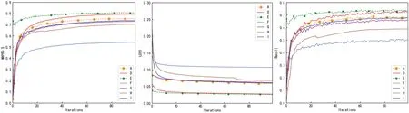
Figure 16:Network average precision,loss function and recall variation curves

According to the experimental results of Model A and Model C in Tables 4 and 5,after adding the small object detection head in this paper,although the computational complexity of the algorithm has increased to some extent,the average detection accuracy and recall rate have improved by 3.33%and 1.88%,respectively.This indicates that the small object detection head plays a crucial role in improving the performance of small object vehicle detection,but it also leads to a more complex model.

Based on the experimental results of Models A and D in Table 6 and Fig.16,it indicates that the lightweight upsampling operator CARAFE introduced in this paper and the addition of a tiny target prediction layer have accelerated the convergence of the network model and improved the average detection accuracy for small vehicle targets.Compared to the original model,the proposed approach increased mAP@0.5 by 4.14%and Recall by 2.17%.Furthermore,it addressed the missed detection problem of small and occluded target vehicles by the network and confirmed the effectiveness of the proposed improvement plan.According to the lightweight comparison analysis presented in Table 5,while the proposed approach slightly increased the network’s parameters and computational complexity,the obtaining improvements in accuracy and detection rates justify this increase.

To achieve model lightweight and reduce the number of parameters and complexity,this article performed channel pruning on network Model D to obtain the final improved model E.The comparative analysis of the lightweight data of Model A and Model E in Table 5 shows that the parameter number of the final improved model E proposed in this article reduced from the original network Model A is 20,871,318 to 7,559,170,a decrease of up to 63.8%.Additionally,the model size is reduced by 24.8 MB,and there is a 31.7 GFLOPS reduction,a decrease of up to 65.8%.

Based on the experimental results presented in Table 6 and Fig.16,it is evident that the improved Model E significantly enhanced the mAP@0.5 from 75.29% to 80.44%,with an increase of 5.15%,thereby improving the detection accuracy of small target vehicles.Moreover,the Recall increased by 4.58%,and the FPS increased from 28 to 47,thereby meeting the requirement of real-time detection speed.Overall,the analysis indicates that the enhanced Model E demonstrates superior detection precision when compared to the original model.The model has removed numerous redundant channels to reduce model complexity and improve performance in small vehicle detection.Additionally,the model has been optimized for real-time detection needs without compromising its lightweight design.

To conduct an in-depth analysis of the enhanced Model E’s detection performance on compact vehicles,other mainstream detection algorithms in the YOLO series were selected for experimental comparison under the same parameters and experimental environment.Based on the experimental findings presented in Table 6 and Fig.16,it can be observed that the average detection accuracy of the improved algorithm increased by 7.52%,10.12%,26.31%,and 6.73% compared to YOLOv5s,YOLOX_s,YOLOv3-tiny,and YOLOv8s,respectively.Furthermore,the network recall rate improved by 7.86%,14.96%,23.74%,and 6.01%,respectively.

Fig.17 provides a comparative analysis of the detection performance of various algorithms on the VisDrone2019-DET dataset.This includes the improved algorithm before pruning,as well as the current mainstream vehicle detection algorithms: YOLOv5m,YOLOv3-tiny,YOLOv5s,YOLOX-s,and YOLOv8s.The x-axis represents the number of images detected per second,with higher values indicating faster detection speed.The y-axis represents the average detection accuracy of the models,with higher values indicating higher average detection accuracy.The ideal position should correspond to the top right corner of the graph,indicating that the model achieves high accuracy while processing images quickly.From the figure,it can be observed that the red dot represents the final improved algorithm.Based on our comprehensive analysis,the improved algorithm outperforms other mainstream detection algorithms in terms of both speed and accuracy.This feature meets the requirements of real-time and lightweight detection without compromising accuracy.It is better suitable for detecting vehicle targets with numerous small targets and substantial differences in scale.The analysis was conducted under the same parameters and experimental environment,making the results reliable and informative.

Figure 17:Comparative analysis of model detection performance

5.5 Comparative Analysis of Detection Effects

Based on the comparative analysis of various evaluation indicators,model E was ultimately determined as the improved model in this paper.Fig.18 displays the original YOLOv5m model’s actual detection effect before improvement,while Fig.19 shows the final improved model’s actual detection effect.The improved model achieves higher detection confidence than the original YOLOv5m model.It successfully detects small and occluded target vehicles that were missed by the original model,further confirming the effectiveness of the proposed improvement solution.

After analyzing the detection results,it was found that the improved model proposed in this paper can more accurately detect small-sized target vehicles at longer distances compared to the baseline model,while also improving the detection speed.However,there are still certain limitations.For example,there are still some instances of missed detections for smaller vehicle targets and dense vehicle targets.

Figure 18:The original YOLOv5m model detection effect

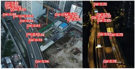
Figure 19:The effect of the improved model detection is shown

6 Conclusion

To address the issues of deep learning technology in the field of vehicle target detection,this paper proposes a lightweight vehicle target detection algorithm based on YOLOv5m.By improving its structure and compressing the model,the average detection accuracy and recall rate were increased by 5.15% and 4.58%,respectively,compared to the original model,and the FPS reached 47.The experiments showed that this enhanced algorithm can accurately detect small and occluded objects in real-time,meeting the requirements of small vehicle detection.Additionally,by cutting redundant channels and parameters,the algorithm greatly compressed the network model,reducing the parameter and computational volume by 63.8% and 65.8%,respectively,and the model size by 24.8 MB.Overall,this algorithm can effectively detect small and dense vehicle targets,providing valuable insights for intelligent city construction.However,the algorithm also has certain limitations and room for improvement.For more complex scenarios,such as small target vehicles with low background contrast,the detection effect is not ideal,which will be a key research topic in the future.

Acknowledgement:The authors would like to thank the anonymous reviewers and the editor for their valuable suggestions,which greatly contributed to the improved quality of this article.

Funding Statement:This research was funded by the General Project of Key Research and Development Plan of Shaanxi Province(No.2022NY-087).

Author Contributions:The authors confirm contribution to the paper as follows: study conception and design:Yaoyao Du and Xiangkui Jiang;data collection:Yaoyao Du;analysis and interpretation of results: Yaoyao Du and Xiangkui Jiang;draft manuscript preparation: Yaoyao Du.All authors reviewed the results and approved the final version of the manuscript.

Availability of Data and Materials:The data that support the findings of this study are openly available at https://github.com/VisDrone/VisDrone-Dataset.

Conflicts of Interest:The authors declare that they have no conflicts of interest to report regarding the present study.