Adaptive Optimal Output Regulation of Interconnected Singularly Perturbed Systems With Application to Power Systems

Jianguo Zhao , Chunyu Yang ,,, Weinan Gao ,,,Linna Zhou , and Xiaomin Liu

Abstract—This article studies the adaptive optimal output regulation problem for a class of interconnected singularly perturbed systems (SPSs) with unknown dynamics based on reinforcement learning (RL).Taking into account the slow and fast characteristics among system states, the interconnected SPS is decomposed into the slow time-scale dynamics and the fast timescale dynamics through singular perturbation theory.For the fast time-scale dynamics with interconnections, we devise a decentralized optimal control strategy by selecting appropriate weight matrices in the cost function.For the slow time-scale dynamics with unknown system parameters, an off-policy RL algorithm with convergence guarantee is given to learn the optimal control strategy in terms of measurement data.By combining the slow and fast controllers, we establish the composite decentralized adaptive optimal output regulator, and rigorously analyze the stability and optimality of the closed-loop system.The proposed decomposition design not only bypasses the numerical stiffness but also alleviates the high-dimensionality.The efficacy of the proposed methodology is validated by a load-frequency control application of a two-area power system.

I.INTRODUCTION

OUTPUT regulation involves designing the controller so that the system output asymptotically tracks a reference trajectory while accommodating an external disturbance,wherein both reference and disturbance signals are generated by an autonomous system [1], [2].In general the design strategies to solve output regulation problems include feedbackfeedforward and internal model principle.The former that tackles output regulation problems is reduced to solve underlying regulator equations [3].In the latter, the output regulation problem is transformed into a stabilization problem of an augmented system consisting of the plant and the dynamic compensator which is constructed based on internal model[4]-[6].For instance, a novel binary distributed observer was imposed in [7] to address the cooperative output regulation problem of heterogeneous linear multi-agent systems (MASs).At present the output regulation problem is broadly treated as a fundamental formulation to deal with numerous control problems of practical dynamic systems such as motors [8],unmanned systems [9], power systems [10], and autonomous vehicles [11], [12].

Optimal control is usually leveraged to improve the transient response of trajectories of the closed-loop control system, wherein the obtained controller minimizes a predefined cost function [13].Meanwhile, reinforcement learning (RL) is a computational intelligence technique, and has been exploited to design adaptive optimal controllers for complex systems with unknown dynamics in the last decade; see e.g., recent papers [14]-[19], surveys [20], [21], tutorials [22], [23], book[24], and the references therein.

To bridge the gap between output regulation and optimality,our prior works [3], [5] stand for the first attempt to combine RL technique, output regulation theory, and optimal control theory to devise feedback-feedforward controllers for linear systems and internal model based distributed controllers for linear MASs, respectively.Since then, a number of RL-based researches have been made on the optimal output regulation problem (O2RP) in the absence of the knowledge of system dynamics.In order to develop an optimal feedback-feedforward controller to solve output regulation problems, two optimization problems are often established to design the feedback and feedforward control parts separately.By small-gain theory, a decentralized optimal output regulator was developed in [25] for leader-follower MASs with unknown interconnections.In [26], an experience-replay-based identification method was proposed for tackling the O2RP over the output matrices being unknown.In [27], two RL-based identification algorithms were further presented for general linear systems.In [28], a convergence rate factor was introduced into cost to assure the convergence rate of the closed-loop system.For the control design via internal model principle, a resilient RL approach was proposed in [6] for partially linear systems against denial-of-service attacks and dynamics uncertainties.By formulating the output synchronization into anH∞optimization problem, an adaptive optimal control method was developed in [29] for heterogeneous MASs.Numerous realworld large-scale systems evolve on multiple time scales due to the coexistence of slow and fast phenomena [30]-[33].Unfortunately, as far as we know, the existing approaches only focus on the O2RP for single-time-scale plants, and there is no available result for multi-time-scale plants either modelbased or data-driven.

Singular perturbation system (SPS) is a powerful tool to character multi-time-scale plants, wherein singular perturbation parameter, a small strictly positive real number, is used to indicate the difference between the time scales of fast and slow states [34].As a consequence, the routine control design ideas are generally no longer suitable because of numerical stiffness and high-dimensionality [35], [36].To this end, a common scheme is to decompose such fast and slow coupling plant into the fast time-scale dynamics and the slow time-scale dynamics and then induce a composite controller through singular perturbation theory (SPT) [37]-[40].Moreover, for a sufficiently small singular perturbation parameter, the stability of the independent fast and slow time-scale dynamics implies the stability of the original system [34].Interconnected SPSs widely appear in chemical engineering, industrial processes, and multi-motor systems.By SPT, one can design a composite decentralized controller to deal with communication constraints in interconnected SPSs, see e.g., [41],[42].For interconnected SPSs with unknown slow dynamics,the RL-based decentralized near-optimal controllers were proposed in [37] and [38] for solving the linear quadratic regulation and tracking problems, respectively.Nevertheless, the existing results on interconnected SPSs neglect the impact of interconnections between fast subsystems on the stability of the overall closed-loop system.

Motivated by the above mentioned observations, we study the adaptive optimal output regulation of interconnected SPSs by combining RL, SPT, and output regulation theory, in which the slow subsystem is unknown and the fast subsystems are interconnected.The main contributions are listed as follows.

1) Unlike single-time-scale systems [1], [2], a composite control framework solving the O2RP is proposed by singular perturbation decomposition.To the best of our knowledge,this article is the first attempt investigating the O2RP of the SPSs, and we rigorously analyze the stability and optimality of the closed-loop systems.

2) He existing works [32], [33], [37], [39], [40] on SPSs only consider interconnections between fast and slow subsystems.To be more realistic, this article further considers the existence of interconnections between fast subsystems and gives the decentralized stabilizable condition of fast time-scale dynamics.

3) A novel off-policy RL algorithm is exploited to learn the optimal control strategy of unknown slow time-scale dynamics.We use the measurement data of the original system to deal with the case that the information of the factitious slow time-scale system is not accessible during learning.Furthermore, the convergence of the proposed learning algorithm is ensured.

4) A real application in the load-frequency control (LFC) of a two-area power system is carried out to validate the proposed theoretical results.

The article is organized as follows.In Section II, the control system with fast and slow states is introduced and the internal model based control strategy is recalled for solving the O2RP.In Section III, main results are presented.We formulate two separate optimization problems associated with the fast and slow time-scale dynamics, which facilitate the decentralized adaptive optimal output regulator design.In Section IV, we illustrate our methodology by simulation results on the LFC in power systems.Concluding remarks are given in Section V.

II.PRELIMINARIES

A. Notations

B. System Description

We consider a class of interconnected SPSs depicted in Fig.1,whose mathematical model is described by

wherez∈Rnzis the slow state,e∈R is the output tracking error,xi∈Rnxiandui∈Rnuiare the state and input of theith fast subsystem, respectively, 0 ＜ε ＜＜1 is the singular perturbation parameter, andv∈Rnvstands for the state of an autonomous system referred as an exosystem

which generates the disturbance signalv, and the reference trajectoryyd=-Fv∈R to be followed by the system outputy=Cz∈R.The minimal polynomial ofSis known andSmay be unknown [3], [5].withnφi=is the interconnection between the fast subsystems.All the matrices are constant with proper dimensions.Throughout this article, three assumptions on the system(1)-(4) are made as follow.

Fig.1.Diagram of the interconnected SPS with x=col(x1,x2,...,xN),which consists of N interconnected fast subsystems in lower layer interconnected through the dynamics of a slow subsystem in upper layer.

Assumption 1: The slow dynamic matricesA00,A0i, andEare unknown.

Assumption 2: The matrixAiiis nonsingular.

Assumption 3: The pair (Aii,Bi) is stabilizable.

Remark 1: The eigenvalues of systems (1) and (2) are clustered into two distinct groups, wherein the dynamics with larger eigenvalues are called fast subsystems and the other is slow subsystem [34].Due to the two-time-scale phenomenon of SPSs, we can also classify the fast and slow states through the rate of state change such as mechatronic systems [8] and industrial processes [38].

Remark 2: Since the fast subsystems are easier to capture and identify than the slow subsystem, it is rational to study the case presumed in Assumption 1 where the slow dynamics are unknown.The standard SPSs satisfy Assumption 2 [34],which is leveraged to decompose the system.WhenAiiis singular, we can first design a fast compensator to stabilize fast subsystem dynamics [43].Then, we proceed to design the composite decentralized adaptive optimal controller.Assumption 3 is a general condition in linear optimal control theory for solving Problem 3.Similar assumptions appeared in the past literature [32], [33], [37]-[40].

C. Review of the Optimal Output Regulation Problem

For convenience, define the vectors to lump the fast states and inputs

In this article, the output regulation problem associated with(1)-(4) is tackled through internal model principle [5], [6].To begin with, we chooseM1∈Rnς×nςandM2∈Rnςsuch that the pair (M1,M2) serves as an internal model ofS.A dynamic compensator is defined as

where ς ∈Rnςrepresents a signal driven by the measurement outpute.Note that, when the characteristic polynomial ofM1is the same as the minimal polynomial ofSand (M1,M2) is controllable, the pair (M1,M2) incorporates an internal model ofS[1].

By [5], [6], one can construct a dynamic feedback controller in the form of

which results in the fact that the closed-loop system (1)-(4)achieves asymptotic output tracking over disturbance rejection if the matrix

is Hurwitz with

For the closed-loop system (1)-(4) under (7), we define the transient variables

where

and the triple satisfies the following regulator equations [1]:

(X,Z,U)

with

then, by the above equations, we have the augmented transient system

which is still an SPS.

In order to improve the transient response of the closed-loop system, an O2RP to design the control gainsKz∈Rnu×nz,Kς∈Rnu×nς, andKx∈Rnu×nxin (7) can be formulated as follows [5], [6].

Problem 1:

whereQz＞0,Qς＞0,Qxi＞0,Ri＞0 are weight matrices.

When the fast and slow characteristics of the system(11)-(13) are disregarded, by [13], the optimal control gains related to Problem 1 are determined by

whereP*＞0 is the solution to the following algebraic Riccati equation (ARE):

with

Remark 3: The controller (7) based on (15) is a centralized control architecture if we directly make use of optimal output regulation theory [5], [6] to the system (1)-(4).In practice,there exist certain constraints such as the privacy protection and the limited communication between fast subsystems,which means that such a controller could not be allowed even though it is an optimal solution to Problem 1.Besides, solving the full-order ARE (16) is subject to numerical stiffness and high-dimensionality due to the coexistence of fast and slow dynamics [35], [36].To bypass these shortages, our objective in this article is to develop a composite decentralized adaptive suboptimal controller to achieve both asymptotic tracking and disturbance rejection under Assumptions 1-3.

III.MAIN RESULTS

In this section, to solve Problem 1, we start with two separate optimization problems for the decoupled fast and slow time-scale dynamics from the system (11)-(13) by singular perturbation decomposition [34].Then, a model-based decentralized optimal control strategy and an RL-based data-driven optimal control strategy are developed for the fast time-scale systems with interconnections and the slow time-scale system with unknown dynamics, respectively.Furthermore, we analyze the properties of the proposed composite decentralized output regulator.

A. Two Separate Optimization Problems

Before proceeding, we define

where κs, κfare used to denote the slow and fast components ofκ, respectively.Note that κfis equal to zero in the slow time scale and κsremains constant in the fast time scale [34].

Setting ε =0 in (13) yields

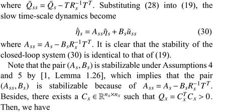
then, using (18) to eliminatex˜ from (11), the slow time-scale dynamics of (11)-(13) are expressed as

where

The substitution of (18) into (14) leads to the following optimization problem for the slow time-scale dynamics.

Problem 2:

where

Two common assumptions are made on the dynamics (19),which ensure the existence of solution to Problems 2.

Assumption 4: The pairis stabilizable.

Assumption 5:

Note that it follows from (19) that:

which possesses multiple input channels withu˜s=col(u˜1s,u˜2s,...,u˜Ns).Therefore, the stabilizability of Assumption 4 can be easily guaranteed as long as one of the input channels makes the above system stabilization.Assumption 5 is a sufficient condition for the solvability of classical output regulation problem.

B. Decentralized Optimal Control Design for Fast Time-Scale Dynamics

Under Assumption 3, by [13], the minimum cost (22)related to (23) is obtained by leveraging the decentralized control

whereKf=blockdiag(K1f,K2f,...,KN f) is given by

andPf=blockdiag(P1f,P2f,...,PN f)＞0 is the unique solution to the ARE

We will then analyze the stability of the fast time-scale closed-loop system consisting of (21) and the decentralized controller (25).The following theorem shows that the interconnected fast time-scale closed-loop dynamics are asymptotically stable under decentralized control.

Theorem 1: For any positive numbersα,β, andγ, suppose thatQx≥αInx,R≤βInu, andDxx≤γInx.Then, the overall fast time-scale closed-loop system (21) with the decentralized control policy obtained from (25)-(27) is asymptotically stable if α ＞γβ.

Proof: Define the Lyapunov candidate

By (25)-(27) and α ＞γβ, along the trajectory of (21), it follows that:

Thus, the fast time-scale system is asymptotically stable.■

Remark 4: By Theorem 1, we can select appropriate weight matricesQxandRfor guaranteeing the closed-loop stability.Similar conditions also appeared in [24].Besides, the condition in Theorem 1 is testable because of the model parameters of fast subsystems being known.

C. Adaptive Optimal Control Design for Slow Time-Scale Dynamics

Now, we are ready to solve Problem 2.In order to convert Problem 2 into a normal form, define

then, we rewrite the cost (20) as

where

For the system (30), by [13], the optimal control policy that minimizes the cost (29) is determined by

wherePs＞0 is the unique solution to the ARE

The key point to capture the optimal control policy (31) is to solve the nonlinear ARE (32).The existing methods usually rely on the knowledge ofAssandBs.However, under Assumption 1, both matricesAssandBsare unknown.This article adopts RL technique [20], [21], [24] to overcome this issue.To this end, we first recall a model-based policy iteration algorithm in the following lemma.

Lemma 1[44]: Given an initial matrix∈Rnx×nusuch that λ(Ass-Bs)∈C-.Letbe the solution to the Lyapunov equation

with

Based on (33) and (34), we derive an off-policy RL algorithm to learn the optimal control policy (31) in terms of measurement data.To begin with, by (1)-(3) and (6), we have the following augmented SPS:

We decompose the system (35)-(37) into fast and slow time-scale dynamics.Let

To formulate the slow time-scale dynamics of (35)-(37), we set ε=0 in (37), solve the resulting equation inxand eliminatexfrom (35) to get

where ηs=col(zs,ςs) andDs=col(E,M2F).The slow component ofxis given by

then, the fast time-scale dynamics are given by removing the slow component fromx

We further rewrite (39) as

with

then, by (33), (34), and (42), we have the following modelfree integral equation:

wheret1andt0are time instants.

Since ηsandussare generated by the factitious system (39),both of their data cannot be directly measured in practice.In order to bypass this obstacle, by (38) and (40), the following behavior policy is considered to excite the system (35)-(37):

with

for all finitet≥0.

Substituting (46a) into (43) yields

meanwhile we define

then, it follows from (47) that:

In other words ηs→η anduss→u¯ssasεtends to zero.

Algorithm 1 Data-Driven RL Algorithm¯K0s =K0s λ(A0ss)∈Cc ＞0 1: Select an initial gain such that and a small 2: Apply (45) on such that (54) holds j ←0[t0,tb]3:4: repeat¯Pjs ¯Kj+1s 5: Solve and from (53)6:j ←j+1|¯Pjs- ¯Pj-1s |＜c 7: until

Remark 5: One way to find a stabilizing control gainis to utilize the knowledge of nominal model parameters.If the slow time-scale dynamics (19) are completely unknown, it is usually desirable to chooseby trial and error.Also, we can also use the hybrid iteration algorithm [6] to obtain such an initial gain in advance.

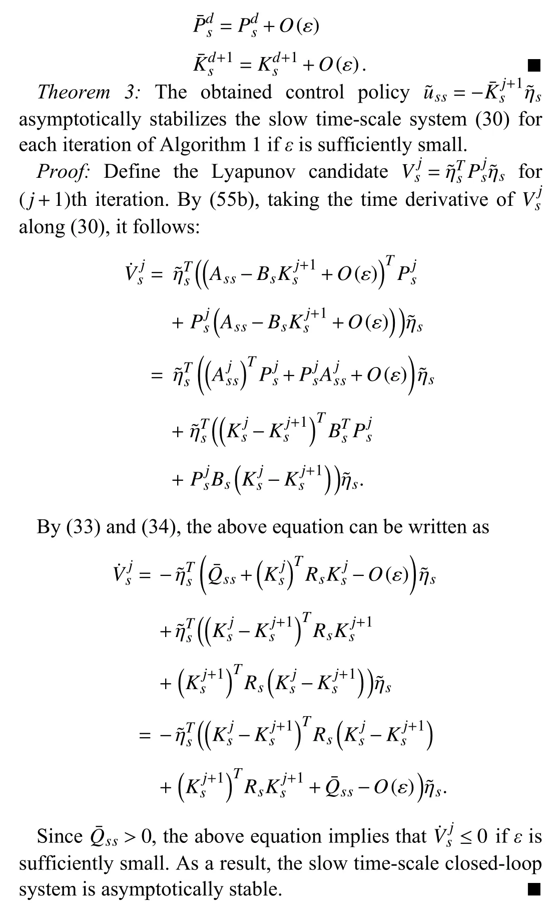
We shall show the convergence of Algorithm 1 and the stability of the slow time-scale closed-loop system (30) withobtained from Algorithm 1 by Theorems 2 and 3.

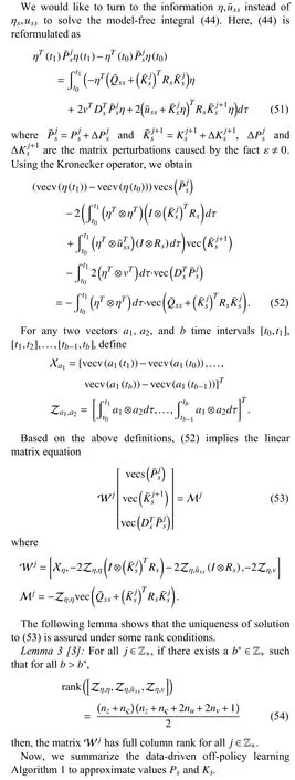
Theorem 2: The sequencesobtained from Algorithm 1 satisfy

Proof: The model-free integral equation (44) is a datadriven version of the model-based algorithm (33), (34) in Lemma 1 [4].In other words, the sequencesdeveloped from (44) are identical to the sequences developed from Lemma 1.Inspired from our previous work [39], we will show the approximation between (51) and (44) to give the proof by an inductive argument.

Forj=0, we haveK¯s0=K0s.By Lemma 2, (47) and (50)hold.Substituting them into (51) leads to

Comparing the above to (44) withj=0, it is easily checked that

Suppose, forj=d＞0, we haveK¯sd=Ksd+O(ε).Then, by(47), (50), and boundedness of matrix norm, equation (51) can be rearranged as

Again, comparing the above equation to (44) withj=d, we have

D. Stability and Optimality Analyses of the Composite Decentralized Output Regulator

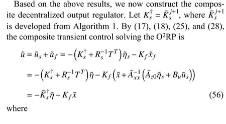
furthermore the composite optimal output regulator is equivalent to

which is a decentralized architecture different from (7), (15).

The following theorem concerns the tracking property and the closed-loop stability for the system (1)-(4) under (57).

Theorem 4: Consider the closed-loop system formed of the system (1)-(4), and the decentralized controller (57).Ifεis sufficiently small and the condition of Theorem 1 holds, then the closed-loop system is asymptotically stable and the output tracking error satisfies l imt→∞e(t)=0.

Proof: It is shown in Theorems 1 and 3 that the slow and fast time-scale dynamics (19) and (21) of the transient system(11)-(13) under (56) are asymptotically stable.According to SPT [34], there exists a scalar ε0such that for any ε ∈(0,ε0],the system (11)-(13) under (56) is asymptotically stable.Therefore, its closed-loop system matrixdeveloped composite controller based on Problems 2 and 3 is a suboptimal control to solve Problem 1, namely,

whereK*is defined in (15).By (60) and (61), we have

Subtracting (16) from (59) yields

whereM=P⊕-P*.By the power series expansion ofMonε,one has

Meanwhile, by (62), it is checkable that

Substituting (64) into (63) and then following the same line of the proof of Theorem 2 in [39], we can obtainMk0=0 andMk1=0,k=1,2,3, because the matricesAss-BsKsandAxx-BuKfare both Hurwitz.As a result, we haveM=O(ε2)which implies (58).■

Remark 6: Compared to the existing learning algorithm [5],the main differences are listed in the following three aspects.Firstly, the time-scale separation approach enables the design of decentralized control structure instead of centralized control.Secondly, the proposed reduced-order model-based control designs reduce the computational complexity of the learning algorithm.Thirdly, our approach is independent of the singular perturbation parameterεand thus bypasses numerical stiffness, which is caused by solving theε-dependent fullorder ARE (16) withεbeing too small.

IV.APPLICATION TO POWER SYSTEMS

Modern power systems are often composed of a number of different generating stations interconnected by transmission networks, which are the so-called multiarea power systems.To balance real-time supply and demand, LFC becomes a critical problem in multiarea power systems with disturbances from loads and generations [45], [46].However, more and more renewable energy sources and new loads (such as plugin electric vehicles) in power systems bring great challenges to frequency stabilization.Consequently, it is very meaningful to study the scenario where the disturbance is time-varying rather than constant for avoiding frequency deviations from the nominal value [10].

In this section we take a two-area interconnected power system that is described in Fig.2 as an application example to verify the efficacy of the proposed methodology by designing a decentralized optimal load-frequency controller over timevarying load disturbance.For mathematical model of annarea power system, the interested readers are referred to[45]-[47].

A. Mathematical Model

Following [45], the dynamic model of each area consisting of governor, turbine, and generator is given by

Fig.2.Structure of the two-area interconnected power system.

whereT12represents the synchronizing power flow coefficient.The tie-line active power deviation exchange satisfies

By [45] and [46], the integral of area control error (ACE) is included into the state vector to achieve frequency deviation synchronization

with

where βirepresents the frequency bias factor.

We consider two interconnected identical areas in this case study.The parameters are specified as follows:Tg=0.1 s,Tt=0.2 s,Mg=10,Dg=0.5,Rd=0.25, β=4.5, andT12=5.2[41].Since the time constants of the governor and the turbine are much smaller than the constants of the generator inertia and the integral control in this model,z=col(Δf1,ΔPtie,1,IACE1,Δf2,IACE2) are taken as the slow states andxi=col(ΔPgi,ΔPti),i=1, 2,as the fast states.According to (1) and(2), we select singular perturbation parameterε=Tt/(Mg/Dg)=0.01.Then,

B. Decentralized Optimal Load-Frequency Controller Design

For each area, our aim is to design a decentralized optimal controlleruithat regulates the frequency deviation Δfito zero despitethetime-varyingload disturbanceΔPdi[10].Suppose thatΔPd1=0.1sintandΔPd2=0.3costinthe interconnected power system.Then, the exosystem dynamics can be described by

it follows from (1) and (3) that:

To fulfill the design requirements, the dynamic compensator in (6) is chosen as

By (19), the slow time-scale dynamics are

Let weight matricesQz,Qς,Qxi, andRiin the cost function(14) be identity matrices.By (26) and (31), the optimal control gains of the fast and slow time-scale dynamics are

Then, by (57), the model-based composite decentralized optimal controller is

C. Simulation Results Using Algorithm 1

In this subsection, the decentralized optimal load-frequency controller is designed based on Algorithm 1 and simulation results are given.

We apply the sum of different frequency sinusoidal signals to excite the interconnected power system.The data is collected fromt=0 s tot=14 s with the sampling interval 0.07 s for Algorithm 1 learning.The convergence ofP¯sjandK¯sjis s hown in Fig.3.It is shown that, under the termination, Algorithm 1 can learn the optimal control gain of the slow time-scale dynamics after five iterations.Then we update the composite decentralized control policy and the trajectories of the frequency deviations and control inputs are shown in Figs.4 and 5, respectively, in which the frequency deviations are capable of regulating to zero.

Fig.3.Convergence of and in Algorithm 1.

D. Simulation Results Using State-Feedback Control Approach

In this subsection, to show the superiority of the proposed methodology, we give the comparative simulation results of the state-feedback control approach without dynamic compensator.

The following state-feedback controller is designed based on pole assignment:

Fig.4.Trajectories of the frequency deviations by our approach.

Fig.5.Evolution of control inputs in Areas 1 and 2 by our approach.

where ζ=col(z,x).The simulation results are given in Figs.6 and 7.It is shown that, compared with our approach, the statefeedback controller has poor frequency regulation performance when the time-varying load disturbance occurs in the power system.

E. Simulation Results Using Existing Algorithm

In this subsection, we provide simulation results for iteratively learning centralized control gain (15) directly using the algorithm of [5].

The data is collected fromt=0 s tot=21 s with the sampling interval 0.07 s during learning.The convergence ofPjandKjis shown in Fig.8.It is shown that, under the termination |Pj-Pj-1|＜0.001, the algorithm of [5] learns the centralized control gain after eight iterations.Compared with our approach, the direct application of [5] requires more learning time and greater computational complexity.

V.CONCLUSION

Fig.6.Trajectories of the frequency deviations by state-feedback control approach.

Fig.7.Evolution of control inputs in Areas 1 and 2 by state-feedback control approach.

Fig.8.Convergence of Pj and Kj in the algorithm of [5].

In this article, a composite decentralized adaptive optimal control framework has been proposed for solving the output regulation problem of interconnected SPSs with unknown slow dynamics by integrating internal model principle, SPT,and RL.By decomposing a predefined quadratic cost function,two separate optimization problems were formulated for fast and slow time scale dynamics, respectively.The fast timescale optimization problem was solved based on model knowledge.On the contrary, the slow time-scale optimization problem was addressed in terms of measurement data.Stability and optimality analyses of the composite adaptive optimal control design were performed using SPT.Finally, the proposed methodology was validated by designing a decentralized optimal load-frequency controller for a two-area power system in the presence of the time-varying load disturbance.

Note that the proposed composite controller design methodology is based on synchronous measurements of full states.For SPSs, the slow state varies much slower than the fast state does.Thus, control designs based on asynchronously sampled measurements may be more computationally efficient, as will be considered in our future work.In addition, considering practical requirements, the output-based feedback control strategy and the case of unknown fast dynamics are also worthy of further study.