Seismic safety assessment with non-Gaussian random processes for train-bridge coupled systems

Zhao Han, Gao Lei, Wei Biao, Tan Jincheng, Guo Peidong, Jiang Lizhong and Xiang Ping

1.Key Laboratory of Geomechanics and Embankment Engineering of Ministry of Education, Hohai University, Nanjing 210024, China

2.School of Civil Engineering, Central South University, Changsha 410075, China

Abstract: Extensive high-speed railway (HSR) network resembled the intricate vascular system of the human body,crisscrossing mainlands.Seismic events, known for their unpredictability, pose a significant threat to both trains and bridges,given the HSR’s extended operational duration.Therefore, ensuring the running safety of train-bridge coupled (TBC) system,primarily composed of simply supported beam bridges, is paramount.Traditional methods like the Monte Carlo method fall short in analyzing this intricate system efficiently.Instead, efficient algorithm like the new point estimate method combined with moment expansion approximation (NPEM-MEA) is applied to study random responses of numerical simulation TBC systems.Validation of the NPEM-MEA’s feasibility is conducted using the Monte Carlo method.Comparative analysis confirms the accuracy and efficiency of the method, with a recommended truncation order of four to six for the NPEMMEA.Additionally, the influences of seismic magnitude and epicentral distance are discussed based on the random dynamic responses in the TBC system.This methodology not only facilitates seismic safety assessments for TBC systems but also contributes to standard-setting for these systems under earthquake conditions.

Keywords: train-bridge coupled (TBC) system; random vibration; new point estimate method (NPEM); seismic safety assessment; moment expansion approximation (MEA); non-Gaussian distributions

1 Introduction

In 2022, a high-speed railway (HSR) network,appearing like blood vessels do throughout the human body, has already spread across the Chinese mainland.Just as blood vessels should remain unblocked, the safety of this train system should be guaranteed.Bridges comprise a large proportion of the HSR lines, especially simply supported beam bridges (Guoet al., 2021).Trainbridge coupled (TBC) vibrations are quite complex under ambient excitations, such as an earthquake occurring when a train is passing across the bridges.An earthquake,as an unpredictable random factor, poses a serious threat to trains and bridges, particularly considering the long operation time of the HSR network (Fig.1).Therefore, seismic reliability analysis for TBC system has gradually become a burning issue (Zhaiet al., 2019).

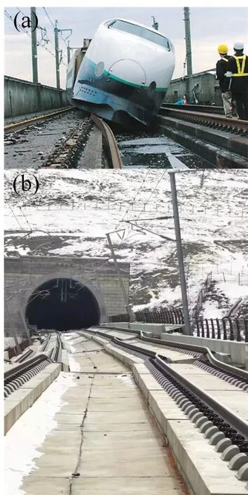
Fig.1 Earthquake-induced damage in TBC systems: (a) derailment of an HSR train on bridges caused by the Niigata Chuetsu earthquake in Japan (Apostolakis et al.,2007; Ogura, 2006; Zhao et al., 2023b); (b) rail bending and track slab cracking resulting from the Qinghai earthquake in China

Earthquakes display strong randomness, such as occurrence location, intensity, soil, frequency, etc.(Wanget al., 2021b).Therefore, it is inevitable that analyzing some random variables with non-Gaussian processes in seismic design must be carried out.The Monte Carlo method (MCM) is a straightforward and primary method to study random responses of TBC systems (Shaoet al.,2023).However, it demands a large number of samples for multivariate analysis, a requirement that presently is unacceptable for a complex system.Instead, many efficient algorithms have been applied to study the random analysis of TBC systems, including the pseudo excitation method (Linet al., 1994), the probability density evolution method (Maoet al., 2016), the new point estimate method (NPEM) (Jianget al., 2019), deep learning (Liet al., 2023; Xianget al., 2023b), and so on.

Different methods are used for various random parameters and problems.Zenget al.(2015a and 2015b)used the pseudo-excitation method to investigate the random vibrations of a high-speed train traversing a slab track on a continuous girder bridge that was subjected to track irregularities and traveling seismic waves.Maoet al.(2016) established a random analysis model for a three-dimensional, high-speed train-track-bridge system subjected to random vehicle load, elastic modulus and mass density of a bridge by use of the probability density evolution method.Later, Liuet al.applied the point estimate method (PEM) and the NPEM to simulate random rail irregularities and calculate the system dynamic response as subjected to Young’s modulus of concrete, damping ratio of concrete, control prestressing stress, and so on (Jianget al., 2019; Liuet al., 2020a).They prove that the PEM and NPEM have excellent computational efficiency and applicability to multiple random variables.On balance, the stochastic method is no longer a bottleneck that restricts the development of random vibration analysis for the TBC system in 2022.In contrast, the mathematical mapping models of the system’s stochastic characteristics and the safety prediction of system response are still not precise enough.

Random distributions of parameters in random analysis are important features that differs from deterministic dynamic analysis.Previously, the vast majority of random parameters in the TBC system obeyed normal or lognormal distribution, such as initial rail irregularities (Liuet al., 2020b), bridge structure parameters (Choet al., 2010; Wanget al., 2021a), train parameters (Tanet al., 2022), and so on.As a result of the high-precision moment formulas and the convenient triple standard deviation method for determining a confidence interval, Gaussian distribution parameters have been extensively studied and exploited regarding random analysis of TBC systems.However, there exist many critical random parameters that satisfy non-Gaussian distribution in seismic analysis, such as seismic magnitude (SM), epicentral distance (ED), etc.(Heet al., 2011).Therefore, a compatible and efficient approach is necessary for seismic safety assessment in TBC systems.

In this paper, the NPEM is applied to fast calculate statistical moments of system responses based on the Gaussian integral method (Jianget al., 2020).Furthermore, the moment expansion approximation(MEA) is introduced to obtain the probability density functions (PDFs) of the system responses based on calculated statistical moments.Thus, the statistics can be deduced according to the obtained PDFs.Consequently,the NPEM combined with the MEA (NPEM-MEA)can solve the probabilistic analysis with non-Gaussian processes.More than that, the NPEM-MEA can be helpful for the standard-setting of TBC systems under earthquakes.In addition, the MEA is applicable to the stochastic methods that can calculate the original moment.

The rest of this paper is organized as follows.

Firstly, random variables, the NPEM, and the MEA are illustrated in Section 2.

Secondly, the TBC system shaken by an earthquake is established in Section 3.

Thirdly, some verifications about the NPEM-MEA in the TBC system are conducted in Section 4.

Fourthly, influences of the two different random parameters on the TBC system are studied in Section 5.

Lastly, several conclusions are drawn in Section 6.

2 Methodology

2.1 Random variables

In this seismic analysis, two critical parameters, SM and ED, are considered as random variables of non-Gaussian distributions, and only strong earthquakes(magnitude equal to or greater than six) are adopted.Specifically, the seismic magnitude-frequency statistics satisfy the truncated Gutenberg-Richter distribution (Jiet al., 2021; Xu and Gao, 2012; Zhaoet al., 2022) in this research, which is a complex exponential distribution.Secondly, the ED herein is assumed to be satisfying uniform distribution because the train could be hit by an earthquake at any location.

The PDF of the truncated Gutenberg-Richter model and the relation between the SM and peak ground acceleration (PGA) of the ground motion attenuation model employed in the paper can be formulated as Eqs.(1) and (3), respectively (Panget al., 2020, 2022;Zhaoet al., 2022).

with

wheret=bl n10,b=0.85;aErepresents seismic PGA;mjmeans the SM;Muare the lower and upper limit of seismic magnitude, which are six and nine, respectively;Reqdenotes the random ED, whose value range is (10 km,100 km);A,B,C,DandEare all regression coefficients of the elliptical attenuation relationship, which are listed in Table 1.The coefficients of the eastern active region are used in this research.

2.2 New point estimate method

The PEM provides a practical solution for reducing computation costs in stochastic analysis (Zhao and Lu,2008, 2021).However, the early PEM’s computational efficiency is still low due to the complexity of structural response functions.Eventually, the PEM was greatly improved so that the NPEM became one of the mainstream estimation methods, by virtue of introducing the reduced dimension method and an approximation model (Caiet al., 2019; Zhao and Lu,2021) to the response function.Nevertheless, it cannot solve a random analysis with a non-Gaussian process.In this connection, this research employs a method that combines the NPEM and the MEA to fill this gap.The details are presented as follows, and the flow chart of the NPEM-MEA is pictured in Fig.2.

First, the distributions of random parameters should be determined and then standardized based on the Nataf transformation (Zhao and Ono, 2000).In this research,the random parameters can be expressed as listed below(Luet al., 2017; Zhaoet al., 2021):

whereXimeans the random variable after the Nataf transformation,Φ( ·) means the standard normal cumulative distribution function,F-1(·) means the inverse function of the cumulative distribution function,andYirepresents the Gauss point of a standard Gaussian distribution.

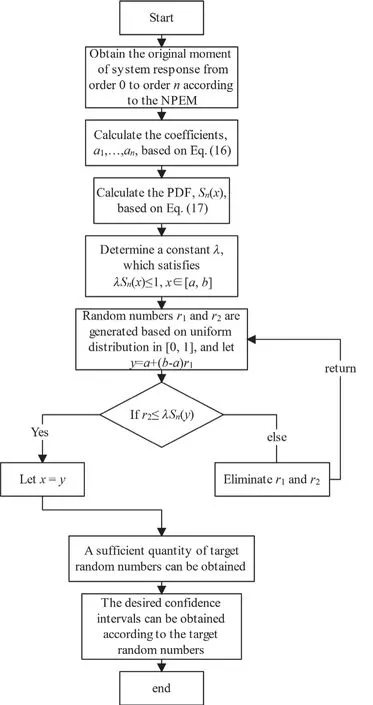
Fig.2 Flowchart illustrating the NPEM-MEA computationalframework

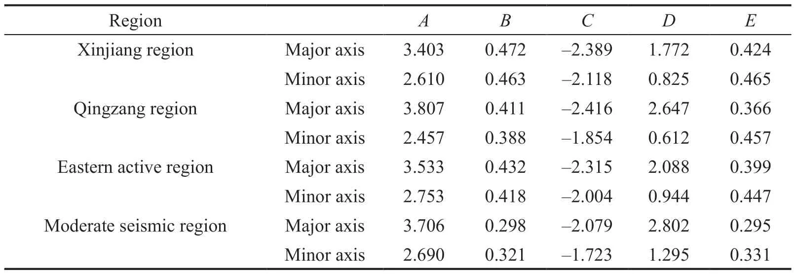
Table 1 Coefficients of the elliptical attenuation relationship of aE for the Chinese mainland(all data can be referred to in Ref.(Zhao et al., 2022))

Second, the number of Gauss pointrand a reference pointμcmust be confirmed, and the reduced dimension method and an approximation model are introduced to solve multiple parameters.For explaining the reduced dimension method, the structural response function containingnrandom variables is assumed ash(x) ,, and a dimension-reduction formula can be expressed as follows (Zhao and Lu, 2021):

wheres＜n,

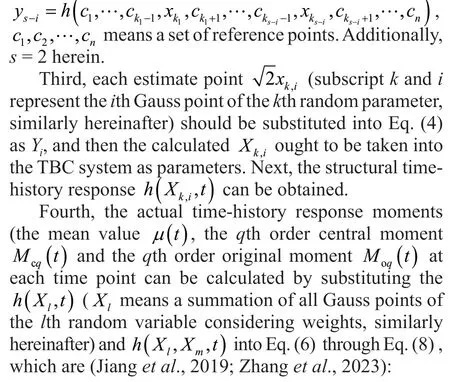
wherenmeans the number of random parameters,h(uc,t) denotes the time-history response when the estimate points are equal to the reference points, and the expectations of some items in Eq.(6) through Eq.(8) are as follows:

whereris the number of estimate points (r= 7 is recommended due to the convenience of obtain upper and lower limits of the random variables for the MEA)andwGH,iandwGH,jare the weights of the Gaussian-Hermite estimate point, which can be refer to in specific literature (Jianget al., 2019; Zhao and Lu, 2021).

When considering a single random parameter, such as thekth random variable, Eq.(6) through Eq.(8) can be rewritten as:

More details of the NPEM can be referred to in monograph (Zhao and Lu, 2021).

2.3 Moment expansion approximation

Statistics required for safety assessment can be obtained according to the PDFs of system responses(Kolassa, 2006).To obtain the PDFs of such responses,the MEA method can be adopted based on the aforementioned moments obtained according to the NPEM.It should be noted that the MEA method is unsuitable for some special random distributions, such as the Cauchy distribution, but these random distributions rarely appear in the field of TBC.

In the MEA method, the best square approximation functionS n(x) of the target PDF,f(x), exists for a given closed interval [a,b] according to approximation theory (Burdenet al., 2015), which can be written as follows:

where ·2means the Euclidean norm.

Then, according to multivariate extremes theory(Castillo, 2012), the normal function can be obtained as expressed below:

where (variable 1, variable 2) means the inner product of variable 1 and variable 2; the polynomial basis of, which are linearly independent of each other, andajare the coefficients to be calculated.

Therefore, Eq.(15) can be rewritten in the matrix form:

whereMoqmeans then-order original moment (original moments can be gained according to Eq.(8) and Eq.(13)calculated by the NPEM).

After the coefficientsa1, …,anare calculated, the best square approximation of the PDF can be described as:

wherendenotes the truncation order of moment expansion.

Subsequently, the obtained PDF allows for the generation of random numbers with a high level of precision.This process can be accomplished using the acceptance-rejection method, and it can be organized as follows (Zhaoet al., 2023c):

3 TBC simulation system

This section presents a system consisting of an ICE-3 train modeled according to multibody dynamics,ballastless track slab models with three layers of elastic point-support, and a finite element bridge model (Fig.3(a)).Additionally, the energy variational method is introduced to calculate matrices in the equation of motion (Lou and Zeng, 2005; Xuet al., 2020).

3.1 Model of train

An HSR train is a three-dimensional vibration system containing an elastic suspension device.For enhanced numerical efficiency, the car-body, bogies, and wheelsets are assumed to be rigid bodies (Xuet al., 2020; Xu and Lu, 2021).Also, the coupler and suspension system of the train are simulated utilizing a three-dimensional linear spring-damper.Each train vehicle has one carbody with six degrees of freedom (DOFs), two bogies with six DOFs each, and four wheelsets with five DOFs apiece (Fig.3).In addition, details and symbols of the basic motions are listed in Table 2.

The detail of the mass matrixMvv, stiffness matrixKvvand damping matrixCvvof the train have the same form as Refs.(Jianget al., 2019; Zhaoet al., 2023b).

3.2 Model of track slab and bridge

As referenced in Figs.4(a) and 4(b), multi-span prestressed HSR simply supported box-girder with concrete piers and China railway track system type Ⅱslab ballastless tracks are adopted for this research,which is modeled based on the finite element method(Gharad and Sonparote, 2021; Xiaet al., 2020; Fenget al.,2020).

Liuet al.(2020a) compared the influence of the Rayleigh damping model and the Caughey damping model and concluded that the Rayleigh damping model is accurate enough to show the dissipation of the system.Therefore, the Rayleigh damping model is adopted for this research, which can be expressed as follows (Zhaoet al., 2023a):

whereiωmeans the first-order natural circle frequency of the bridge,jωmeans the second-order natural circle frequency of the bridge, andbζrepresents the damping ratio of the bridge.

3.3 Model of wheel-rail contact

The spatial geometric relationship of wheelrail (WR) contact can be calculated according to the monograph (Zhai, 2020), and the schematic diagram is shown in Fig.4(c).

The coordinate of the WR contact point in the absolute coordinate system can be deduced as:

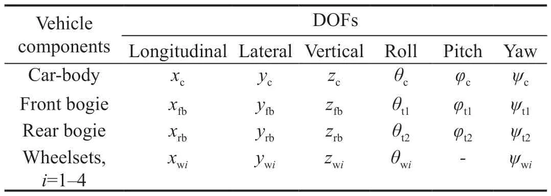
Table 2 DOFs of the train

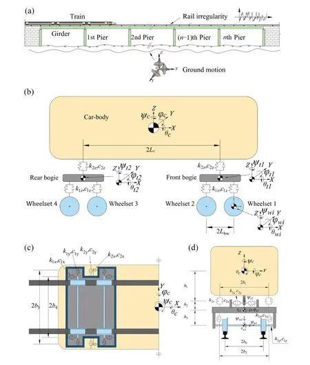
Fig.3 Schematic representation of the TBC system: (a) overall system, (b) side view, (c) top view and (d) front view of the train vehicle model

with

where

Rδmeans the contact angle of the right wheel tread;

wRdenotes the rolling radius of the wheel;

l x,l y,lzare the direction cosines of thex-axis,y-axis,z-axis, respectively;

x B,y B,zBrepresent the coordinates of the center of the wheel rolling circle;

dwmeans the abscissa of the wheel rolling circle in the wheel coordinate.

The WR normal force can be solved by using the nonlinear Hertz elastic contact theory (Guoet al., 2023).The WR creep force is formulated according to the Shen-Hedrick-Elkins nonlinear model (Xu and Zhai, 2017).Additional details of the WR contact geometries and forces can be found in the monographs (Kalker, 1990;Zhai, 2020).

3.4 Model of rail irregularity

The influence of primary rail irregularity on dynamic train response has been considered.The rail irregularities in the TBC system are generated according to German low disturbance power spectral density (PSD), based on the harmonic synthesis method (Chenet al., 2013; Jianget al., 2019), which can be expressed as:

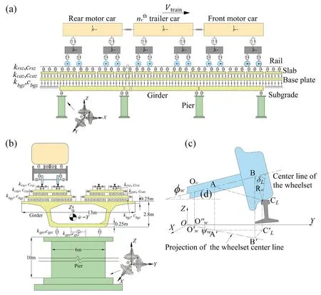
Fig.4 Diagrams depicting (a) the side view and (b) rear view of the bridge model, along with (c) the WR contact model

whereSv,Sa, andSgare the irregularity PSD function of vertical rail profile, rail alignment and gauge distance,respectively m2/(rad/m);

Scis the PSD function of rail cross-level irregularity 1/(rad/m);

Av,Aa, andAgrepresent roughness coefficients;

Ωc,ΩrandΩsembody truncation frequencies;

andbdenotes the half distance between two sides of the rail.

The detailed parameters of the irregularity PSD function are shown in Table 3.The vertical rail profile irregularity of the left railrZLand right railrZR, and alignment irregularity of left railrYLand right railrYRcan be referred to in literature (Jianget al., 2019).

3.5 Model of an earthquake

Only a far-field earthquake is adopted for this research, and the Clough-Penzien PSD functions are used to simulate the seismic wave sample, which has a form of (Zenget al., 2015b; Zhanget al., 2011):

Table 3 Parameters of German low disturbance PSD of rail irregularity (all data refer to Zhai (2020))

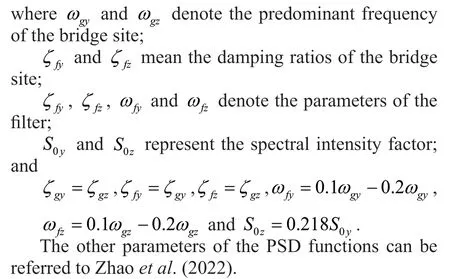
Seismic wave has obvious non-stationarity of intensity.Hence, it is described as a product of a stationary filtered wave and a time-varying function in engineering applications (Shinozuka and Sato, 1967),that is:

with

3.6 Motion equation

In the TBC system, the earthquake loads are treated as external excitations, and the acceleration input mode is adopted.Specifically, it is assumed that the bridge piers are connected to the ground through the supporting nodes.Meanwhile, the dynamic equation of the system is partitioned, as supporting nodes block matrix(supporting nodes) and other structures block matrix(structure nodes) in the absolute coordinate system,which can be expressed as follows (Chopra, 1995; Sunet al., 2016; Zhaoet al., 2023a):

where:

Xbmeans the enforced displacements of the supporting nodes;

Xsrepresent the displacements of structure nodes;

Mss,CssandKssare the mass matrix, damping matrix, and stiffness matrix of the structure nodes,respectively;

Mbb,CbbandKbbare the mass matrix, damping matrix, and stiffness matrix of the supporting nodes,respectively;

Msb,Mbs,Csb,Cbs,KsbandKbsdenote the coupling mass matrices, the coupling damping matrices,and the coupling stiffness matrices of the supporting nodes and the structure nodes;

fbis the force of the supporting nodes subject to the ground.

The first row of Eq.(27) is expanded based on the lumped mass assumption, and it can be calculated that:

whereXsis decomposed into pseudo-static displacementYpsand dynamic displacementYd, namely:

The pseudo-static displacementYpssatisfies static equilibrium (set dynamic displacements, all velocities and accelerations to zero), henceYpscan be deduced as follows (Chopra, 1995):

Naturally, the pseudo-static velocity and acceleration can be obtained based on Eq.(30):

In particular, the damping force is considered to be proportional to the dynamic velocityYd′, so Eq.(28) can be transformed into:

Afterward, considering Eqs.(31) and (32) ignoring the damping force of the supporting nodesCsbXb′,Eq.(33) can be recast as:

In the system, the acceleration of the earthquake is uniformly input for each bridge pier.Thus, the motion equation of the system can be expressed as follows:

whereXg′(t) represents the earthquake acceleration of all support nodes in three directions.

4 Verification

In this section, a relatively simple system has been established (Fig.5(a)), as the low computational efficiency of the MCM.First, an ICE-3 train with two motor vehicles and one trailer vehicle (MTM) is applied.Its main parameters are listed in Table A1.Second, a fivespan 32 m prestressed HSR two-way, simply supported box-girder bridge is established based on Section 3.2.The main parameters of the track slab and bridge are listed in Table A2.Third, primary rail irregularities are generated by the use of German low disturbance PSD functions (Section 3.3).Also, a set of three-dimensional artificial seismic waves is adopted (Fig.5, Secion 3.5).Lastly, the train ran a short distance (about 50 m) before crossing the bridge, and maintained a constant speed(200 km/h) until leaving the bridge.The ground motion is loaded exactly at the instant when the train enters the bridge.

4.1 Verification of random variables

To verify the feasibility and efficiency of each random variable calculated by the NEPM-MEA, a series of calculations are accomplished according to NPEM-7 and MCM-1000 (the numbers mean the number of Gauss points adopted for NPEM and calculation times for MCM, respectively).Thereafter, the comparison of the 3rd car-body response between the MCM-1000 and the NPEM-7 from the 1st to 4th order moment is applied to validate the method.As the topmost unit of the TBC system, the findings are convincing enough to verify the acceleration of the car-body rather than the remaining part of the system.

Fig.5 (a) The schematic diagram of the TBC model, (b, d, f) three-dimensional seismic acceleration time-history curves and(c, e, g) the pertinent PSD curves of the three components

Figure 6 compares the acceleration time history of the 3rd car-body in the lateral and vertical directions between the NPEM-7 and the MCM-1000, with random SM.The horizontal axis in each subgraph denotes the distance of the first wheelset passing through the start point.It can be observed that the NPEM-7 curves and the MCM-1000 curves all agree well with one another in both directions and in each subgraph.Furthermore,the simulation results demonstrate that even the 4th central moment, as calculated by the NPEM-7 is still accurate.Regarding calculation efficiency, the NPEM-7 outperforms MCM-1000 by two orders of magnitude in this simulation.

Similarly, Fig.7 compares the acceleration time histories of the 3rd car-body in the lateral and vertical directions between the NPEM-7 and the MCM-1000,with random ED.Figure 8 compares the acceleration time-histories of the 3rd car-body in the lateral and vertical directions between the NPEM-7 and the MCM-1000, with both random variables.Consistent results in all the subgraphs displayed in Figs.7 and 8.This consistency confirms that the accuracy of the NPEM-7 is sufficient for different random variables with non-Gaussian distribution characteristics.

4.2 Optimal truncation order of moment expansion

The moments calculated by the NPEM become increasingly inaccurate as the order of moments increases(Jianget al., 2019).Therefore, there is an optimal value for the truncation order of the MEA method.Thereafter,the PDF curves at several randomly selected time points in the 3rd car-body acceleration under MCM-1000 and the NPEM-MEA with different truncation orders are used to find the optimal value.

Different PDF curves of the 3rd car-body acceleration presented in Fig.9 are generated by the MCM-1000 and the NPEM-MEA, with a truncation order from three to eight in two directions (lateral and vertical) calculated at two points of time (distance = 139 m and distance = 60 m)and with different random variables.The different time points and directions shown in Fig.9 are chosen randomly for generality.Wherein the PDF curves of MCM-1000 are generated byksdensityfunction, a built-in function in MATLAB (used version: R2020b), which uses a kernel smoothing function for estimating univariate or bivariate data.More details can be found in MATLAB help files.This type of probability density estimation method has a significant error at the boundary of the domain, which explains the dropping part (inaccurate part) at the end of the MCM-1000 curves.However, the remainder of the curve is sufficiently accurate (Bowman and Azzalini,1997).For comparing the PDF curves among different truncation orders, the Euclidean distance approach is introduced, and it is modified as follows to satisfy the demands of this research:

Fig.6 Comparative analysis of the 3rd car-body’s acceleration time-history curves between NPEM-7 and MCM-1000 with random SM: (a) mean value, (b) variance, (c) third moment, and (d) fourth moment in the lateral direction (y-direction,similarly hereinafter); (e) mean value, (f) variance, (g) third moment, and (h) fourth moment in the vertical direction(z-direction, similarly hereinafter)

wherey1(i) andy2(i) are theithvertical coordinates of the two curves, which have the same abscissa;nmeans there arenpoints on the curve with equal abscissa spacing,andnis large enough to ensure accuracy.

Naturally, the smaller the Euclidean distance is, the closer are these two curves, according to Eq.(36).In Fig.9,the MCM-1000 curves are considered to comprise target curves (in addition to the inaccurate part), and the calculated Euclidean distances are listed in Table 4.By comparison, it can be observed that the NPEM-MEA curves are all close enough to the MCM-1000 curve in each subgraph, but the proximity of these NPEM-MEA curves to the target curves shows a slight difference.Specifically, the NPEM-MEA curves ofn= 5 and 6 are closest to the MCM-1000 for Figs.9(a) and 9(d);the NPEM-MEA curves ofn= 3 and 4 correspond to Figs.9(b) and 9(e); and the NPEM-MEA curves ofn=4 and 5, correspond to Figs.9(c) and 9(f).Therefore, the optimal truncation order of the NPEM-MEA will change with the random variable, but four to six are accurate enough for the truncation order.

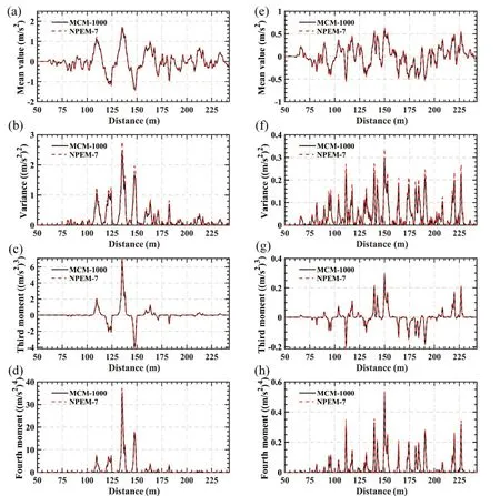
Fig.7 Comparative analysis of the 3rd car-body’s acceleration time-history curves between NPEM-7 and MCM-1000 with random ED: (a) mean value, (b) variance, (c) third moment, and (d) fourth moment in the y-direction; (e) mean value, (f) variance,(g) third moment, and (h) fourth moment in the z-direction

Figure 10 compares acceleration probability curves of the 3rd car-body generated by the MCM-1000 and the NPEM-MEA with a truncation ordern= 6 in the vertical direction, with both random variables and at different confidence levels.In addition, the confidence interval curves include the upper and lower curves, and the space between the two curves has a specific probability, which is the confidence level, containing the true value.The confidence interval curves for estimating the response of the TBC system at any designated confidence level can be obtained by means of the NPEM-MEA.However, a confidence level with guiding significance for seismic design results from careful consideration of economics,safety and many other factors, which is still blank at present, will not be studied herein.Therefore, two randomly chosen confidence levels (0.6 and 0.8) are used to validate the confidence interval curves that are generated based on the NPEM-MEA by comparing them with the MCM-1000.According toSecondly, the TBC system shaken by an earthquake is established in Section 3.0, it can be found that the upper and lower curves are almost coincident at both confidence levels.In addition,the computing time of the MEA method is about five minutes (used MATLAB version: R2020b, used CPU:Intel Core i7-10700), and it is negligible compared to the computing time of the NPEM.

5 Safety assessment

A much more complex model can be evaluated within an acceptable computing time according to the NPEMMEA with multiple non-Gaussian distribution random variables.Therefore, a seven-span, simply supported beam bridge and a train consisting of two motor vehicles and two trailer vehicles (MTTM) are adopted (Fig.12(a)).Also, the other system’s parameters are consistent with Section 4, except that the train’s speed is 250 km/h.Thereafter, Figs.12 and 13 depict the lateral and vertical acceleration time-history curves of the 4th car-body at the three confidence levels, with random SM and ED,respectively, as well as the displacement of the 4th span midpoint.

5.1 Influence of a single random variable

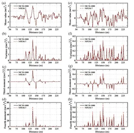
Fig.8 Comparative analysis of the 3rd car-body’s acceleration time-history curves between NPEM-7 and MCM-1000 with both random SM and ED: (a) mean value, (b) variance, (c) third moment, and (d) fourth moment in the y-direction; (e) mean value,(f) variance, (g) third moment, and (h) fourth moment in the z-direction

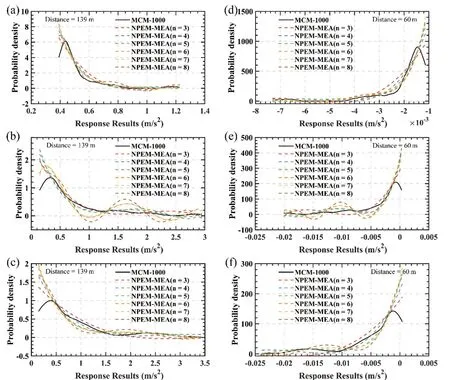
Fig.9 PDF curves of the 3rd car-body acceleration between the MCM-1000 and the NPEM-MEA with truncation orders from three to eight: (a, b, c) for the time point (distance = 139 m) in the lateral direction (SM, ED, both); and (d, e, f) for the time point (distance = 60 m) in the vertical direction (SM, ED, both)

Table 4 Euclidean distance among different curves

It is impractical to build the HSR railway bridge,which can withstand an earthquake of extreme intensity,considering construction difficulties and attendant economic effects.Since earthquakes cannot be predicted at present, Figs.12, 13, and 14 can evaluate the response range of the TBC system from the perspective of probability.Additionally, according to vibration criteria for HSR bridges and train vehicles in China (Xiaet al.,2018; Xianget al., 2023a), it is recommended that a car-body’s lateral and vertical acceleration not to exceed 1.3 m/s2and 1.0 m/s2, respectively.In addition, the lateral displacements of the bridge midpoints should be limited to 3.5 mm.Accordingly, the over-limit area will be considered a dangerous space, and the remaining area will be judged to be safe (Guoet al., 2010).On this basis, three confidence levels are chosen to evaluate the reliability of the TBC system, by which the 0.99 confidence interval curves can be considered the extreme state.

In Fig.12, it can be seen that for the train, three confidence interval curves exceed its limits in the lateral direction.Meanwhile, the vast majority of the 0.6 area (confidence interval curves enclose the pertinent confidence level areas) is within the safe area in the lateral direction of the bridge.It is found that train running safety is threatened in more than half of the cases when a single random SM is considered.Another finding is that the train and the bridge are much safer in the vertical direction.This particular phenomenon indicates that train running safety is more vulnerable than is the case with the bridge itself.

Conversely, a different situation is displayed in Fig.13.Three confidence level areas exceed the safe area for both the train and the bridge in the lateral and vertical directions.Therefore, the train and the bridge are highly likely to become damaged with a single random ED.Further, the train exhibits a high probability of strong vibration in the vertical direction.

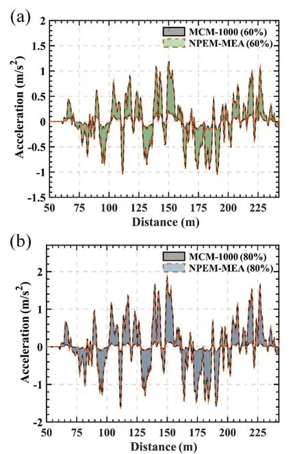
Fig.10 Acceleration probability curves of the 3rd car-body generated by the MCM-1000 and the NPEM-MEA with truncation order n = 6 in the vertical direction with both random variables for several confidence levels: (a) 0.6, and (b) 0.8

5.2 Influence of both random variables

Figure 14 shows the lateral and vertical acceleration time-history curves of the 4th car-body at the three confidence levels, with both random SM and ED,as well as the displacement of the 4th span midpoint.Subsequently, the standard deviation (Std.D)timehistory curves of the train and bridge responses with each random variable are depicted in Fig.15.

Figure 14 shows that all three confidence level areas seriously exceed the limits for the train and the bridge in both directions.These results reveal a much more dangerous set of circumstances compared to the simulation results with a single random variable, as shown in Figs.12 and 13.Consequently, an earthquake as a multivariate control system demonstrates a character of high randomness.With regard to seismic reliability analysis, it is necessary to simultaneously consider the randomness of multiple vital parameters.According to Fig.15, the uncertainty in the dynamic response of the TBC system under the effects of an earthquake can be divided and allocated to different random variables.It can clearly be observed that the Std.Dtime-history curves of ED are consistently above the curves of SM for the train and the bridge in both directions at any time point when the train is passing across the bridge.There is no doubt that the ED has greater influence than the SM on the response of the train and the bridge.

Fig.11 Schematic diagram of the TBC model

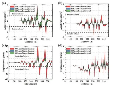
Fig.12 Train and bridge response safety assessment curves under seismic excitations with the random SM: 4th motor car-body in the (a) y and (b) z directions; 4th span midpoint in the (c) y and (d) z directions

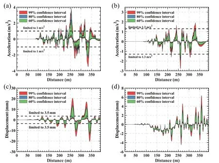
Fig.13 Train and bridge response safety assessment curves under seismic excitations with the random ED: 4th motor car-body in the (a) y and (b) z directions; 4th span midpoint in the (c) y and (d) z directions

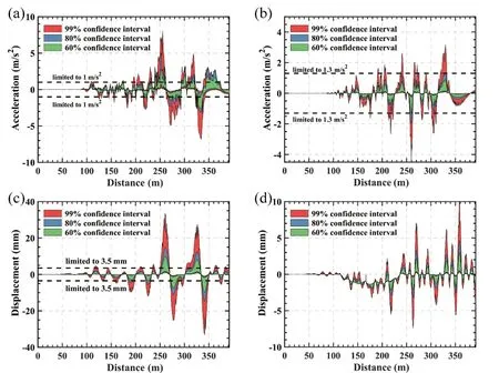
Fig.14 Train and bridge response safety assessment curves under seismic excitations with both the random SM and ED: 4th motor car-body in the (a) y and (b) z directions; 4th span midpoint in the (c) y and (d) z directions

Fig.15 Std.D time-history curves of the train and bridge response with both the random SM and ED: 4th motor car-body acceleration in the (a) y and (b) z directions; 4th span midpoint in the (c) y and (d) z directions

6 Conclusions

This research investigated a seismic safety assessment in an established three-dimensional TBC system with non-Gaussian distribution parameters based on the NPEM-MEA.The NEPM-MEA is verified by comparing it with the simulation results taken from the MCM.A safety assessment of the train and bridge under both random variables is discussed.The main conclusions of the study are as follows:

(1) The NPEM-MEA demonstrates a high degree of accuracy in the seismic safety assessment of the TBC system with non-Gaussian distribution variables,verified by comparing it with the MCM results.In terms of calculation efficiency, the NPEM-7 is two orders of magnitude higher than the MCM-1000.

(2) The recommended truncation order of the NPEM-MEA is 5 or 6 for the random SM, 3 or 4 for the random ED, and 4 or 5 for both SM and ED.The optimal truncation order of the moment expansion will change with different stochastic methods and random distributions of parameters.In addition, four to six will be sufficiently accurate for the truncation order of the NPEM-MEA.

(3) Train running safety is more vulnerable than for the bridge in the lateral direction, and train running safety is threatened in more than half of the cases when considering a single random SM.However, both the train and the bridge are much safer in the vertical direction.

(4) The train and the bridge have a high probability of being damaged, considering random ED.Additionally,the train shows a high probability of strong vibration in the vertical direction, which would seriously affect train running safety.The randomness of ED has a greater influence than that of SM on the response of the train and the bridge in both directions at any time point when the train is passing across the bridge.

(5) From the perspective of probability and the limit state, the responses of the train and the bridge with random SM and ED are significantly higher than those having a single random variable.This highlights the importance of considering the randomness of multiple parameters simultaneously in seismic safety assessment.