Direct scaling of residual displacements for bilinear and pinching oscillators

Mohammad Saifullah and Vinay K.Gupta

Department of Civil Engineering, Indian Institute of Technology Kanpur, Kanpur 208016, India

Abstract: The estimation of residual displacements in a structure due to an anticipated earthquake event has increasingly become an important component of performance-based earthquake engineering because controlling these displacements plays an important role in ensuring cost-feasible or cost-effective repairs in a damaged structure after the event.An attempt is made in this study to obtain statistical estimates of constant-ductility residual displacement spectra for bilinear and pinching oscillators with 5% initial damping, directly in terms of easily available seismological, site, and model parameters.None of the available models for the bilinear and pinching oscillators are useful when design spectra for a seismic hazard at a site are not available.The statistical estimates of a residual displacement spectrum are proposed in terms of earthquake magnitude,epicentral distance, site geology parameter, and three model parameters for a given set of ductility demand and a hysteretic energy capacity coefficient in the case of bilinear and pinching models, as well as for a given set of pinching parameters for displacement and strength at the breakpoint in the case of pinching model alone.The proposed scaling model is applicable to horizontal ground motions in the western U.S.for earthquake magnitudes less than 7 or epicentral distances greater than 20 km.

Keywords: residual displacement spectrum; bilinear hysteresis model; pinching hysteresis model; nonlinear analysis;scaling model

1 Introduciton

The evolution of performance-based earthquake engineering during the past 20-30 years has been closely associated with a growing emphasis on the accurate and convenient estimation of residual displacements under seismic excitations.Residual displacements represent permanent deviations in structural configurations due to hysteretic energy dissipation during the seismic response of inelastic systems.Those are well-correlated with structural damage caused during earthquake events and therefore must be limited to carry out costfeasible repairs in damaged structures.Those residual displacements may need to be limited even further in cost-effective solutions that factor into businessinterruption costs.If residual displacements are measured following an earthquake event, those can be used in the post-earthquake assessment of damage, and thereby the ability of a structure to withstand future earthquake events.

Starting with the pioneering work by Mahin and Bertero (1981), several studies have focused on the estimation of residual displacement in the case of singledegree-of-freedom (SDOF) systems and have made important contributions in the understanding of the relative roles played by possible governing parameters in residual displacements.MacRae and Kawashima (1997)showed that mean residual displacements normalized by the maximum possible residual displacements significantly depend upon the post-yield stiffness ratio in the case of bilinear systems.Kawashimaet al.(1998)proposed mean normalized residual displacement spectra for different values of post-yield stiffness ratio.Borziet al.(2001) and Christopouloset al.(2003) showed that residual displacements normalized with respect to maximum inelastic displacements increase with an increase in ductility and post-yield softening ratio for bilinear oscillators.Christopouloset al.(2003) further showed that the normalized displacements are much smaller for the self-centering hysteresis model compared to the Takeda and bilinear models.Ruiz-Garcia and Miranda (2006) proposed a predictive equation for residual displacement spectra normalized by maximum elastic spectral displacement in the case of elasticperfectly plastic (EPP) oscillators.They observed that site conditions can have a significant effect on the mean residual displacement spectra.Further, Ruiz-Garcia and Guerrero (2017) showed a sharp decline in normalized residual displacements for the oscillator periods close to the predominant period of ground motion in the case of soft soil conditions.Liossatou and Fardis (2015) proposed the mean and 0.9-fractile residual displacement spectra normalized with respect to elastic and inelastic spectral displacement spectra for the Bouc-Wen hysteresis model.A more comprehensive review of the studies up to 2020 has been presented by Saifullah and Gupta (2020).In the latter studies, Amiriet al.(2021) introduced a normalized residual index for predicting residual displacements of mainshock-damaged structures during subsequent aftershocks, while proposing constant-strength spectra for a bilinear hysteretic model.Seyed Ardakaniet al.(2021) developed constant-ductility residual drift spectra for RC bridge columns under near-fault ground motions by considering different displacement ductilities, site conditions, and one-second spectral acceleration levels.Zhanget al.(2022) presented a probability-based model for predicting normalized residual displacements in single-degree-of-freedom systems, while highlighting significant dispersion due to variations in model parameters and ground motion characteristics.

It has been common to study the dependence of residual displacements on various governing parameters after being normalized with respect to maximum possible residual displacements (MacRae and Kawashima, 1997;Kawashimaet al., 1998), maximum elastic displacements(Ruiz-Garcia and Miranda, 2006; Harikrishnan, 2009;Liossatou and Fardis, 2015; Harikrishnan and Gupta,2020a, 2020b; Saifullah and Gupta, 2020), or maximum inelastic displacements (Mahin and Bertero, 1981; Borziet al., 2001; Christopouloset al., 2003; Harikrishnan,2009; Liossatou and Fardis, 2015; Harikrishnan and Gupta, 2020a, 2020b; Amiriet al., 2021; Zhanget al., 2022) in the oscillator.The predictive equations developed in the course of these studies can be useful provided that seismic hazard at the site of interest has been characterized in terms of inelastic or elastic response spectra.Harikrishnan (2009) and Harikrishnan and Gupta (2020a) therefore attempted a direct scaling of constant-ductility residual displacement spectra in terms of earthquake magnitude, epicentral distance, and site geology parameter.This scaling model is, however,applicable only for the EPP oscillators.Considering that the EPP model may not truly represent the hysteretic behavior of most realistic structures, it would be useful to consider the direct scaling of (constant-ductility)residual displacement spectra in the case of hysteresis models that can capture realistic situations more accurately.These models should incorporate all modes of degradation in stiffness and strength that are observed in experimental results.

This study considers the direct scaling of residual displacement spectra for the pinching and bilinear hysteresis models proposed by Ibarraet al.(2005)for RC and timber structures, and steel structures,respectively.While the pinching model proposed by these authors incorporates energy-based cyclic degradation mechanisms and has been calibrated with experimental data of RC columns and plywood shear walls on the hysteresis energy dissipated for various loading protocols, the bilinear model proposed by them demonstrates a more realistic post-capping behavior.Their pinching model is preferred over the Bouc-Wen-Baber-Noori hysteresis model (Baber and Noori, 1985)because it has fewer governing parameters, and thus lesser uncertainty associated with the estimation of model parameters.For bilinear and pinching models,the statistical estimates of constant-ductility residual displacement spectra are directly obtained in terms of easily available seismological, site, and model parameters.First, the dependence of the constantductility residual displacement spectrum on various seismological, site, and model parameters, as well as strong-motion duration, is explored for an ensemble of ground motions to ascertain whether and how the considered parameters govern residual displacements in the mean sense for different time-frequency characteristics of ground motions.Second, based on identified governing parameters and the observed dependence of the mean residual displacement spectrum on those parameters, a scaling model is proposed for the two hysteretic models.Third, regression analyses are conducted for the proposed scaling model by considering a suite of 1,076 horizontal ground motions that were recorded in western U.S.Smoothed regression coefficients are obtained for 46 discrete periods, and errors in the estimation of the residual displacement spectrum are modeled for those periods for varied levels of confidence.Finally, a parametric study is carried out to illustrate how the residual displacement spectrum for a given level of confidence depends upon various governing parameters.

2 Residual dispalcements

2.1 Hysteretic models

The bilinear and pinching models used in this study contain a backbone curve proposed by Ibarraet al.(2005) and considered by Saifullah (2018) (see Fig.S1 in Supplementary Materials).This is a commonly used multilinear hysteretic backbone and is similar to that proposed and used for moment-curvature relation (Yang and Lu, 2018; Luet al., 2018).This curve is governed by the following parameters: (1) elastic stiffnessKe; (2)yield strengthFy; (3) post-yield stiffnessKh(=αhKe),whereαhrefers to the post-yield strain hardening ratio;(4) post-capping stiffnessKc(=αcKe), whereαcrefers to the post-capping stiffness ratio; (5) yield deformation levelδy(=Fy/Ke); (6) deformation level at capping point,δc; (7) strengthFcat capping point, expressed asFy+Kh(δc-δy); (8) residual strengthFr(=λFy), whereλrefers to the residual strength ratio (taken as zero in this study,assuming that no residual strength is left at collapse);and (9) the parameterδr, defined asδc+(Fc-Fr)/Kc.The two models differ from each other with regard to their basic hysteresis rules, as described in detail by Saifullah (2018).The hysteresis rule for the pinching model is characterized by the pinching parameters for displacement and strength, i.e.,kdandkf, respectively,which are defined to establish the break points in the hysteresis curve.However, the basic hysteresis rules for the bilinear model have no break points, and thus the pinching parameterskdandkfplay no role in the hysteresis curve of the bilinear model.The strength and stiffness degradation mechanism for the two models comprises cyclic degradation, which depends upon the dissipated hysteretic energy in a cycle and the remaining hysteretic energy capacity of the system through a parameter defined in terms of dissipated hysteretic energy in that cycle, as well as the hysteretic energy capacity coefficientγ, which can be experimentally calibrated (Saifullah, 2018).

The parameterFyis determined iteratively such that the maximum displacement ofδisμtimesδy(=Fy/Ke).Thus, the independent model parameters for the pinching model areαh,αc,δc/δy,γ,kd, andkf, while those for the bilinear model areαh,αc,δc/δy, andγ, for a given set of ductility ratioμ, periodT, and the initial damping ratio.The hysteresis cycles obtained for the bilinear and pinching models considered in this study are illustrated in Figs.1(a) and 1(b), respectively, in the case of the N21E component of the motion recorded at Taft Lincoln School tunnel during the 1952 Kern County earthquake.The oscillator that is considered has the following parameters: periodT= 0.5 s, ductility ratioμ= 4,αh= 0.1,αc= -0.1,δc/δy= 2.3,γ= 100 for both bilinear and pinching models, andkd=kf= 0.5 in the case of the pinching model.In both figures, the values of forceF(= -oscillator mass × ground acceleration) applied to the oscillator mass and displacementδof the oscillator mass are normalized with respect to the yield forceFyand yield displacementδy, respectively.

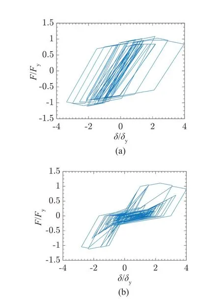
Fig.1 Hysteresis cycles for (a) bilinear and (b) pinching models with μ = 4, T = 0.5 s, αh = 0.1, αc = -0.1, δc/δy = 2.3, γ = 100 and kd = kf = 0.5, under Kern County motion

2.2 Residual displacement spectrum

The residual displacementurof a base-excited SDOF system is defined as a permanent shift in the mean position, about which the oscillator mass oscillates after the removal of the excitation.The governing equation of motion for such a SDOF system with a unit oscillator mass is given as:

whereζrepresents the initial damping ratio,ωn(= 2π/T)is the (initial) natural frequency of the oscillator,k(u) is the oscillator stiffness governed byu(t) and the type of hysteresis, andu˙˙g(t) is the base acceleration.A residual displacement spectrum,ur(T) , describes the variation of the magnitude of the residual displacementurwith the oscillator periodTfor a given constant ductility ratio(or for a given lateral strength ratio).It may be useful to observe how the residual displacement spectrum varies with the input ground motion for the two types of oscillators that are considered.For this purpose, six ground motions (with their details provided in Table 1)are considered.The (constant-ductility) residual displacement spectra are computed for each of these motions in the case of the bilinear and pinching models by consideringαh= 0.1,αc= -0.1,δc/δy= 2.3,γ= 100,kd=kf= 0.5, and 5% initial damping.There are 46 periods considered as follows: 0.2, 0.22, 0.24, 0.26, 0.28, 0.3,0.32, 0.34, 0.36, 0.38, 0.4, 0.42, 0.44, 0.46, 0.48, 0.5,0.55, 0.6, 0.65, 0.7, 0.75, 0.8, 0.85, 0.9, 0.95, 1, 1.1, 1.2,1.3, 1.4, 1.5, 1.6, 1.7, 1.8, 1.9, 2, 2.2, 2.4, 2.6, 2.8, 3,3.2, 3.4, 3.6, 3.8, and 4 s.The Newmark-beta integration technique with linear acceleration is used with the timestep Δtof 0.0005 s for the integration of Eq.(1).The given ductility demandμ, which refers to the ratio of the maximum displacementumaxof the oscillator to its yield displacementuy, is achieved by iterating the lateral yield strength such that the target and computed ductility demands differ by less than 1%.Further, the residual displacements are computed by adding a sufficient number of zeroes at the end of the accelerogram to bring the oscillator to a complete rest.

Figures 2(a) and 2(b) show the residual displacement spectra forμ=4 in the case of the bilinear and pinching models, respectively.Each figure shows six such spectra for the six ground motions that are considered.It may be observed that residual displacements vary arbitrarily within wide ranges, particularly at longer periods, from ground motion to ground motion, and that the pinching model is associated with significantly larger residual displacements.Further, there are no trends with regard to the variation of residual displacement with oscillatorperiod for a given ground motion.This indicates that the residual displacements are arbitrarily sensitive to oscillator periods.

Table 1 Details of example ground motions considered for studying variations of the residual displacement spectrum with input ground motion

The six ground motions considered above differ significantly from each other with respect to their time-frequency characteristics, as determined by the patterns of arrivals of different seismic waves, as well as their energy distributions.It will therefore be useful to first ensure that all the six motions conform to the same elastic response spectrum prior to comparing the corresponding residual displacement spectra.To this end, the six considered ground motions are made compatible with the 5%-damping USNRC pseudo spectral acceleration (PSA) spectrum proposed by USAEC (1973) for a 1.0 g peak ground acceleration(PGA), as shown in Fig.3.The ground motions are made compatible by using the wavelet-based procedure of Mukherjee and Gupta (2002).Subsequently, those are filtered through a 4th-order Butterworth band-pass filter with cut-offfrequencies of 0.0375 Hz and 20.75 Hz and then subjected to a quadratic type baseline correction.

The residual displacement spectra computed for these ground motions are shown in Figs.4(a) and 4(b),respectively, for the bilinear and pinching models.One obvious effect of making the six ground motions compatible with the same response spectrum appears to be that theur(T) spectra for the two models are now much closer.This implies that the differences between the residual displacements of the bilinear and pinching models depend significantly on the shape of the response spectrum.The two models may respond similarly or one of those may lead to much larger residual displacements,depending upon the shape of the response spectrum.Further, the residual displacement spectrum appears to be more sensitive to the type of hysteretic nonlinearity than to the characteristics of the ground motion (both in terms of energy distribution and time-frequency characteristics).It is also obvious from the comparison of the spectra in Figs.2(a) and 4(a), as well as in Figs.2(b)and 4(b), that for a given model the differences between theur(T) spectra for different ground motions are primarily due to their time-frequency characteristics; the differences in their response spectra appear to play a less significant role.Figures 4(a) and 4(b) also confirm that the variations in residual displacements with oscillator periods or ground motions are arbitrarily sensitive to the patterns of wave arrivals in the ground motions.It may be noted, however, that despite large fluctuations, everyur(T) spectrum shown is associated with a rise in its mean level with period.

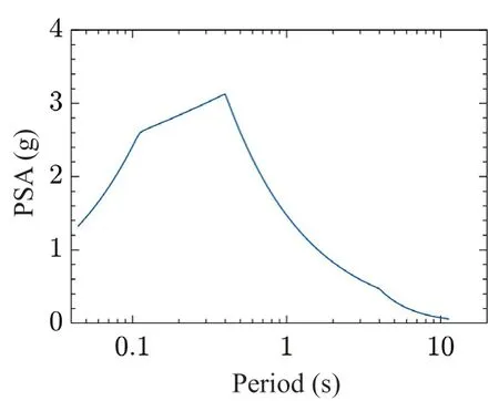
Fig.3 5%-damping USNRC (PSA) spectrum for 1.0 g PGA

The sensitivity of the residual displacement response to the pattern of wave arrivals in the ground motion that was mentioned above leads to uncertainty regarding how differently the oscillator of a given period will respond to various ground motions with the same response spectrum or how differently the oscillators of different periods will respond to the same ground motion.This uncertainty also exists in the response of oscillators having different values of a model parameter other than the period, as illustrated in the case of the ductility ratioμfor the bilinear and pinching oscillators that were considered above, under the Kern County ground motion.Figures 5(a) and 5(b) show the comparisons of theur(T)spectra forμ= 3, 4, 5 in the case of the bilinear and pinching oscillators, respectively.It may be observed that there are no consistent trends for both models with respect toμat any period.However, since the residual displacements are higher for largerμvalues at most periods, consistent trends are likely to exist in theur(T)spectra averaged for an ensemble of ground motions.These observations are consistent with those reported in Harikrishnan (2009) and Harikrishnan and Gupta(2020b) for the elastic-perfectly-plastic oscillators.

3 Dependence of ur(T) on various parameters

In this section and subsequent sections, a scaling model is developed for the bilinear and pinching hysteretic models for a direct estimation of the constantductility residual displacement spectrumur(T) in terms of the specified seismological, site, and model parameters in the case of horizontal ground motions.The seismological and site parameters considered are earthquake magnitude, epicentral distance, geological site condition parameter, and strong-motion duration(SMD).The model parameters considered are post-yield strain hardening ratioαh, post-capping stiffness ratioαc,peak displacement to yield displacement ratioδc/δy, and hysteretic energy capacity coefficientγfor both bilinear and pinching models, and the pinching parameters for displacement and strength at the break point,kdandkf,for the pinching model alone.

For a direct scaling of residual displacements,it is desirable to determine whether and how these displacements depend on the plausible governing parameters.It has been shown by Saifullah (2018)in the case of bilinear and pinching oscillators that residual displacements normalized by elastic spectral displacements do not show significant variations with earthquake magnitudeM, epicentral distanceR, and geological site condition parameters.However, the elastic spectral displacements are known to significantly depend upon various seismological and site parameters.Also, Harikrishnan (2009) and Harikrishnan and Gupta(2020a) found the residual displacements to depend uponM,R, andsin the case of EPP oscillators.Therefore, the possible dependence of residual displacements onM,R, andsis considered in this study.The dependence on SMDTsis also explored, since it may be an important parameter in the case of stiffness degradation.Further,based on the dependence of normalized residual displacements observed by Saifullah (2018) on the parameters of the bilinear and pinching oscillators,the possible dependence of the residual displacements on parametersαh,αc,δc/δy, andγ, is explored.The dependence on pinching parameterskdandkfis not considered and both parameters are assumed to be equal.

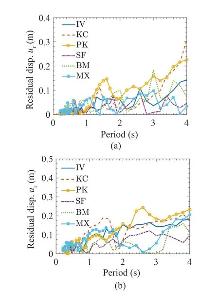
Fig.4 Residual displacement spectra for (a) bilinear and(b) pinching models with μ = 4, αh = 0.1, αc = -0.1,δc/δy = 2.3, γ = 100 and kd = kf = 0.5, under spectrumcompatible Imperial Valley (IV), Kern County (KC),Parkfield (PK), San Fernando (SF), Borrego Mountain (BM), and Michoacan (MX) motions

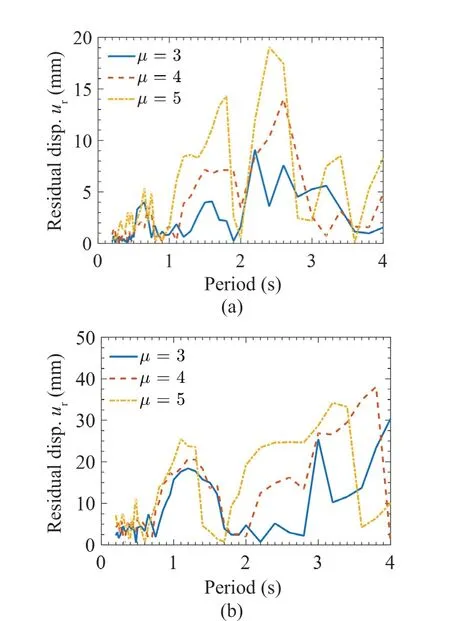
Fig.5 Comparison of residual displacement spectra for(a) bilinear and (b) pinching models with μ = 4, αh = 0.1,αc = -0.1, δc/δy = 2.3, γ = 100, kd = kf = 0.5 and different ductility ratios under Kern County motion

3.1 Dependence on seismological and site parameters

The residual displacements at a period have significant and random variations from one ground motion to another, even when the ground motions conform to the same (elastic) response spectrum, as shown by Harikrishnan (2009) and Harikrishnan and Gupta (2020b) for constant-ductility EPP oscillators.The constant-ductility bilinear and pinching oscillators(with model parameters remaining unchanged) also show such behavior, as noted in the previous section.This happens because the residual displacements are highly sensitive to the pattern of wave arrivals and to the resulting time-frequency characteristics of the ground motion.As discussed by Saifullah (2018), this can be addressed by considering the statistical estimates of residual displacements obtained for an ensemble of motions instead of the estimates for a single ground motion.Therefore, 25 ground motions were arbitrarily selected from a suite of 259 strong motions recorded during 14 earthquake events in the western U.S.A.between 1931 and 1984, which were obtained from the entire database of motions described by Lee and Trifunac (1987) by discarding the ground motions with peak ground accelerations (PGAs) less than 0.15 g.For the motions in this suite, earthquake magnitudesMs range between 4.5 and 6.9, epicentral distancesRs vary from 4 to 62 km, strong-motion durationsTss(as per the definition by Trifunac and Brady (1975)) range between 1.8 s and 42 s, and site conditions vary from alluvium to rock.The selected 25 motions (for details, see Table S1 in Supplementary Materials) are made compatible to the 5%-damping PSV spectrum proposed by Trifunac and Lee (1985b) (for a given set ofM,R,H, ands), as described in the previous section, to provide ensembles of 25 ground motions for different sets ofM,R,H, ands.The (fixed) model parameters are taken as follows:αh= 0.1,αc= -0.1,δc/δy= 2,γ= 100,kd,f= 0.5 (withkd,fbeing the abbreviation forkd=kf),μ= 4, and the initial damping ratio = 5%.In this study, this is referred to as the base case.

The different sets ofM,R,H, andsconsidered are as follows: (a)M= 4, 5, 6, 7, 8, withR= 20 km,H=5 km, ands= 2 (hard rock site conditions) for studying the dependence upon earthquake magnitude; (b)R= 5,20, 50, 75, 100, 150 km, withM= 6,H= 5 km, ands= 2(hard rock site conditions) for studying the dependence upon epicentral distance; and (c)s= 0 (alluvium site conditions), 1 (intermediate site conditions), 2 (hard rock site conditions), withM= 6,R= 20 km, andH=5 km for studying the dependence upon geological site conditions.For a given set ofM,R,H, andsvalues, the values of the mean residual displacementurare calculated for the natural periodT= 0.25, 0.5, 1, 2 s, with the model parameters remaining fixed.This is done by taking the average of the residual displacements computed for the 25 motions of the relevant ensemble (for the given set ofM,R,H, andsvalues) in each of the four cases ofTvalues.Figures 6(a)-6(c) show the variations of the logarithm of the meanurwith earthquake magnitudeM, epicentral distanceR, and site geology parameters,respectively, for the four values of periodTin the case of the bilinear model.Similarly, Figs.7(a)-7(c) show the variations of the logarithm of meanurwith earthquake magnitudeM, epicentral distanceR, and site geology parameters, respectively, for the four values of periodTin the case of the pinching model.It may be observed from Figs.6(a) and 7(a) that the logarithm of meanurincreases parabolically withMfor both the bilinear and pinching models, which can be considered to be linear for magnitudes ＜ 7.It will be seen later that the suite of ground motions considered for the regression analysis has few records forM＞ 7, and thus it will be reasonable to assume a linear variation of meanurwithMfor this study.Similarly, there are few (near-fault) records forR＜ 20 km, and thus, the variations of the logarithm of the meanurwithRshown in Figs.6(b) and 7(b) may be assumed to be linear for all four periods.Further,Figs.6(c) and 7(c) indicate that the logarithm of meanurdecreases linearly, as we proceed from alluvium site conditions (s= 0) to hard rock site conditions (s= 2).

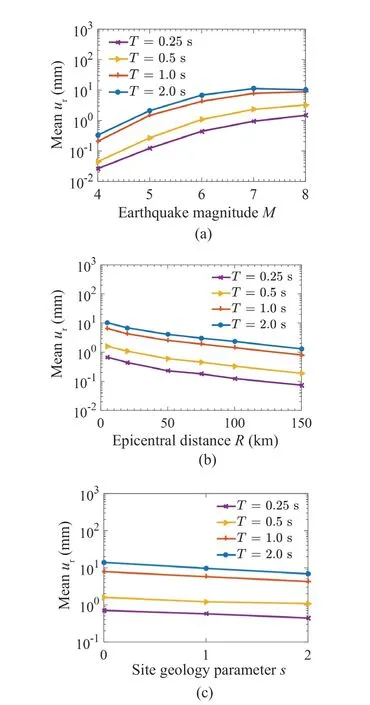
Fig.6 Variations of logarithm of mean residual displacement with (a) earthquake magnitude M, (b) epicentral distance R, and (c) site geology parameter s at different periods for the bilinear model with μ = 4,αh = 0.1, αc = -0.1, δc/δy = 2, γ = 100

3.2 Dependence on strong-motion duration

To study the dependence on SMDTs, several bins with significant variations in the mean SMD and with a reasonably large number of records in each of those are required, and thus a larger set of ground motions is considered.The set of 956 horizontal ground motions recorded during the 106 earthquake events in the western U.S.A.region from 1931-1984 (see Lee and Trifunac (1987) and Tiwari and Gupta (2000) for further details) is considered and made compatible with the 5%-damping PSV spectrum proposed by Trifunac and Lee (1985b) forM= 7,R= 20 km,H= 5 km, and hard rock site conditions (s= 2), as described in the previous section.This leads to five bins of 46, 40, 30, 37, and 55 modified motions havingTsvalues, according to the SMD definition of Trifunac and Brady (1975) within±5% of 10, 20, 30, 40, and 50 s, respectively.The mean c onsidered in the previoussectionfor eachof thesebinsur(T)spectra are calculated forthesame46 periodsas by averaging theur(T) spectra obtained for the 46, 40,30, 37, and 55 modified motions (corresponding to bins of 10, 20, 30, 40, and 50 s, respectively) for both bilinear and pinching models (with the model parameters remaining fixed at their base values).The coefficient of variation (COV) values also are computed from theur(T) spectra (at the 46 periods) for each of these cases.Figures 8(a) and 8(b), respectively, show the meanur(T)spectra and COV spectra for the central SMD values of 10, 20, 30, 40, and 50 s in the case of the bilinear model.Similarly, Figs.9(a) and 9(b), respectively, show the meanur(T) spectra and COV spectra for the five central SMD values in the case of the pinching model.

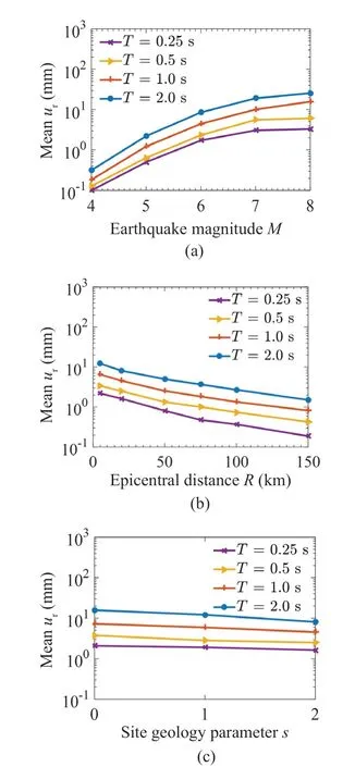
Fig.7 Variations of logarithm of mean residual displacement with (a) earthquake magnitude M, (b) epicentral distance R, and (c) site geology parameter s at different periods for the pinching model with μ = 4,αh = 0.1, αc = -0.1, δc/δy = 2, γ = 100 and kd,f = 0.5

Figures 8(a) and 9(a) indicate the absence of a consistent pattern in how residual displacements vary with the central SMD values at any period for both models.Further, the COV values are large, as observed in Figs.8(b) and 9(b), and thus, even though there are ranges of periods (e.g., those up to 1.5 s in the case of the pinching model) where the five curves are close to each other, there can be large random variations in residual displacements calculated for the periods in these ranges irrespective of the values of SMD.For the same reason,it may not be reasonable to account for (in the scaling model for residual displacements) the observation that mean residual displacements are largest for the motions with SMDs around 10 s for the periods up to 1.7 s for the bilinear model and longer than 0.9 s for the pinching model.Further, it may be observed from Figs.8(b) and 9(b) that the curves for different central SMD values differ little from one another and in an inconsistent manner irrespective of the oscillator model, and that the bilinear model is associated with about 50% more COV values compared to the pinching model.This implies that the uncertainty in how an oscillator (of a given period) responds to a given ground motion in respect of its residual displacement is not governed by the SMD of the motion, and that this uncertainty is greater for the bilinear model.Besides depending upon the type of oscillator model considered, this uncertainty is also governed by the parameters of the model, as shown by Saifullah (2018).In view of these observations, the dependence of meanur(T) spectrum on SMD is ignored in this study for both the bilinear and pinching models.

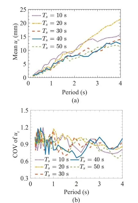
Fig.8 Comparison of (a) mean and (b) COV spectra of residual displacement ur for the bilinear model with μ = 4, αh = 0.1,αc = -0.1, δc/δy = 2, γ = 100, under ground motions with different central SMD values, and M = 7, R = 20 km,H = 5 km, s = 2

3.3 Dependence upon model parameters

To explore the dependence of residual displacement for a given period on various model parameters, a single ensemble of 25 ground motions is generated from the 25 recorded motions considered above, such that those motions are compatible with the PSV spectrum proposed by Trifunac and Lee (1985b) forM= 6,R= 20 km,H=5 km, and hard rock site conditions (s= 2).Further, each of the parameters that are considered, i.e.,αh,αc,δc/δy,andγ, is varied while keeping the other parameters the same, as in the base case described above.Different values of the parameter being varied are listed as follows:αh= 0.01, 0.05, 0.1, 0.15, 0.2, 0.25, 0.3;αc=-0.01, -0.05, -0.1, -0.15, -0.2, -0.25, -0.3;δc/δy=1.2, 1.5, 2, 3, 4; andγ= 30, 50, 75, 100, 200, 300.For a given value of the parameter being varied, the values of the mean residual displacementurare calculated for the natural periodT= 0.25, 0.5, 1, 2 s by taking the average of residual displacements for the 25 motions of the ensemble generated above in each of these four cases.Figures 10(a)-10(d) show the variations of a logarithm of the meanurwith post-yield stiffness ratioαh, post-capping stiffness ratioαc, peak displacement to yield displacement ratioδc/δy, and the hysteretic energy capacity coefficientγ, respectively, for the four values of periodTin the case of the bilinear model.Similarly,Figs.11(a)-11(d) show the variations of logarithm of the meanurwithαh,αc,δc/δy, andγ, respectively, in the case of the pinching model.

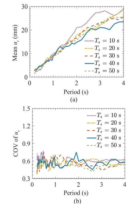
Fig.9 Comparison of (a) mean and (b) COV spectra of residual displacement ur for the bilinear model with μ = 4, αh = 0.1,αc = -0.1, δc/δy = 2, γ = 100, and kd,f = 0.5 under ground motions with different central SMD values, and M = 7,R = 20 km, H = 5 km, s = 2

Fig.10 Variations of logarithm of mean residual displacement with (a) post-yield stiffness ratio αh, (b) post-capping stiffness ratio αc, (c) peak to yield displacement ratio δc/δy, and (d) hysteretic energy capacity coefficient γ of the bilinear model for different periods under ground motions with M = 6, R = 20 km, H = 5 km, s = 2

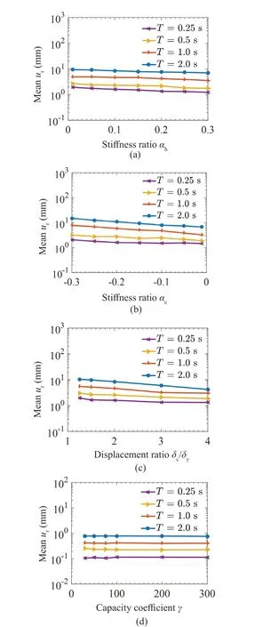
Fig.11 Variations of logarithm of mean residual displacement with (a) post-yield stiffness ratio αh, (b) post-capping stiffness ratio αc, (c) peak to yield displacement ratio δc/δy, and (d) hysteretic energy capacity coefficient γ of the pinching model for different periods under ground motions with M = 6, R = 20 km, H = 5 km, s = 2

It may be observed from Figs.10(a) and 11(a) that the logarithm of meanurdecreases almost linearly withαhfor both the bilinear and pinching models.However,the rate of decrease is much smaller in the case of the pinching model and is higher at the lower values ofαh.These observations are consistent with the behavior of the meanCr(T) value (at periodT) withαh, as observed by Saifullah (2018).Figures 10(b) and 11(b) similarly indicate a nearly linear increase in the logarithm of meanuron increasing the magnitude ofαc, with the rate of increase being slightly higher for the bilinear model and very small at short periods for the pinching oscillators.These observations are also consistent with the behavior of the meanCr(T) value (at periodT) withαc, as observed by Saifullah (2018).The variations of the logarithm of meanurwithδc/δy, as shown in Figs.10(c) and 11(c),can also be considered linear, even though the rate of decrease in this (with an increase inδc/δy) decreases for the higher values ofδc/δyin the case of bilinear model.Figure 11(c) also shows the trend observed by Saifullah (2018) that the sensitivity of the logarithm of the meanurdecreases for shorter periods in the case of pinching oscillators.Figures 10(d) and 11(d) confirm the observation made by Saifullah (2018), that the meanurvalue can be considered independent of the parameterγ, with the other governing parameters remaining unchanged, for both the bilinear and pinching models.

4 Scaling model and database

Based on the linear variations observed in the logarithm of the meanurby varying each of the seismological and site parameters,M,R, ands, and model parameters,αh,αc, andδc/δy, the following scaling equation is attempted for the (mean) residual displacement spectrumur(T) in the case of both the bilinear and pinching models:

Here,bi(T)’s are period-dependent coefficients obtained for a ductility demand ratioμin the case of the bilinear model, and for a set ofμand model parameterskd,fin the case of the pinching model.To determine these coefficients by regression, a dataset of 1,076 horizontal ground motions are considered.This database consists of(a) 956 accelerograms recorded during 106 earthquake events in the western U.S.between 1931 and 1984, with the details given in Lee and Trifunac (1987), and (b) 120 accelerograms recorded during the 1994 Northridge earthquake (for details, see Table S2 in Supplementary Materials).For a bilinear model with the givenμ,or for a pinching model with a given set ofμandkd,f, 1,076 sets of the model parametersαh,αc, andδc/δyare randomly generated to be used together with the 1,076 ground motions on a one-on-one basis, withαhranging from 0.01 to 0.3,αcfrom -0.01 to -0.3, andδc/δyfrom 1.5 toμ.The distributions of the values ofαh,|αc|, andδc/δyof the 12 sets of the so-generated 1,076 random combinations in different sub-intervals of these ranges (ofαh,αc, andδc/δy) are shown in Tables S3-S5,respectively, in Supplementary Materials.The value ofγis taken uniformly equal to 100 for all such sets of model parameters.The residual displacements are computed at 46 periods (which were listed in the previous section)for each of the 1,076 sets of ground motion and model parameters (withμandkd,fremaining fixed).

Table 2 shows the distribution of the 1,076 ground motions considered among different magnitude ranges(i.e., 3-3.9, 4-4.9, 5-5.9, 6-6.9, and 7-7.9), with the data in each magnitude range further sub-divided into the bins of different site conditions (i.e., alluvium,intermediate, or rock) and epicentral ranges (i.e.,R≤100 km andR＞ 100 km).It may be observed that this database has an uneven distribution of data, with a heavy bias towards the 6-6.9 magnitude bin, with about 52%motions showing up in this bin.Also, about 72.6%motions belong to the alluvium site conditions andR≤100 km.It will not be appropriate to provide the same weightage for all of the 1,076 motions in the regression analysis, and therefore the generatedurdata is sieved through sorting as in Trifunac and Anderson (1977,1978) and Trifunac and Lee (1978, 1985a, 1985b)in order to minimize possible bias in the regression coefficients to be computed.To this end, theurdata (for a combination of period and fixed model parameters)for the 1,076 motions sub-divided into 30 sub-bins, as shown in Table 2, is arranged in decreasing order for each sub-bin.This is done, provided that the sub-bin corresponds toR≤100 km and there are more than 19 motions in the sub-bin, or that the sub-bin corresponds toR＞ 100 km and there are more than 5 motions in the sub-bin.In the former case, 19urvalues corresponding to the 5, 10, …, 95 percentiles are selected from the ordered data.In the latter case, 5urvalues corresponding to thepercentiles are selected.For the other sub-bins, all theurvalues are considered for the regression analysis.Thus, there are 239 sets of data points on which the regression analysis in this study is based.Table 2 lists the breakdown of these 239 sets in different sub-bins.It may be mentioned that this selection process screens out theurvalues corresponding to different ground motions for various combinations of period and fixed model parameters, and thus theurdata for all 1,076 ground motions is utilized in the regression analysis.This process also addresses the limitation thaturvalues for individual ground motions are used, even though the proposed scaling equation pertains to the residual displacements averaged over several ground motions.

5 Regression analysis

Regression analysis is carried out for all of the 46 periods forμ= 3, 4, 5 in the case of the bilinear model and for the nine combinations ofkd,f= 0.25, 0.5, 0.75 andμ= 3, 4, 5 regarding the pinching model.The so-obtained least-square estimates of the regression coefficientsbi(T),i= 1, 2, …, 7 are represented bybˆi(T),i= 1, 2, …, 7.In the following cases of the pinching model these estimates of the regression coefficients are found to be positive and near-zero in magnitude: (a)μ= 3,kd,f= 0.25,b6ˆ(T) forT≤ 0.6 s, andb7ˆ(T) forT≤ 0.3 s;(b)μ= 3,kd,f= 0.5,b4ˆ(T) forT≤ 0.22 s,b6ˆ(T) forT≤ 0.4 s, andb7ˆ(T) forT≤ 0.24 s; (c)μ= 3,kd,f= 0.75,b4ˆ(T) andb6ˆ(T) forT= 0.2 s; (d)μ= 4,kd,f= 0.25,b4ˆ(T) forT≤ 0.28 s, andb6ˆ(T) forT≤ 0.3 s; (e)μ= 4,kd,f= 0.5,b4ˆ(T) forT≤ 0.26 s, andb6ˆ(T) forT= 0.2 s;(f)μ= 4,kd,f= 0.75,b4ˆ(T) andb6ˆ(T) forT≤ 0.22 s;and (g)μ= 5,kd,f= 0.5,b4ˆ(T) forT= 0.2 s, andb6ˆ(T) forT≤ 0.24 s.Since these cases of positive values ofb4(T) ,b6(T) , andb7(T) are inconsistent with decreasing trends of the logarithm of the meanurwith the parameterss(see Fig.7(c)),αc(see Fig.11(b)), andδc/δy(see Fig.11(c)), respectively, the relevant values ofb4(T) ,b6(T) , andb7(T) are forced to be zero and the remaining regression coefficients are recomputed from the reduced forms of the scaling equation in Eq.(2).It may be observed that the step of forcingb4(T) to take zero values is consistent with the observation made in Fig.7(c) that the rate of decrease in the logarithm of the meanur, as one moves from alluvium to hard rock site conditions, is minimum at the shorter periods.Similarly,forcingb6ˆ(T) andb7ˆ(T) to be zero is consistent with the “near-constant” values of meanurin Figs.11(b) and 11(c), respectively, forT= 0.25 s.The least-square estimates of the regression coefficients (including the recomputed values) are smoothed along the periodTaxis by using the 5-point linear Savitzky-Golay filter in MATLAB.The values ofb4(T) ,b6(T) , andb7(T) forced to be zero above are restored to the zero values after the process of smoothing.The process of smoothing takes care of the random variations between the mean residualdisplacements of the oscillators of two different periods.The smoothed least-square estimates,7, of the regression coefficients at 17 selected periods are shown in Tables S6-S8 in Supplementary Materials for the bilinear oscillators withμ= 3, 4, and 5, respectively.These estimates are furnished in Tables S9-S11 in Supplementary Materials for the pinching oscillators withμ= 3, 4, and 5, respectively in the case ofkd,f=0.5.For the pinching oscillators withkd,f= 0.25 and 0.75, the smoothed least-square estimates of the regression coefficients are provided in Tables S12-S17 in Supplementary Materials.

The smoothed least-square estimates,3, …, 7, shown in Tables S6-S17, are consistent with the observed variations of logarithm of the meanurwith the six governing parameters shown in Figs.6(a)-6(c),7(a)-7(c), 10(a)-10(c), and 11(a)-11(c).For example,b2ˆ(T) is consistently positive andb3ˆ(T) is consistently negative for both types of oscillators.This is in agreement with the increasing meanurwithM, as shown in Figs.6(a) and 7(a), and with the decreasing meanurwithR, as shown in Figs.6(b) and 7(b).Further, higherb2ˆ(T) values for shorter periods are consistent with the observation made in Figs.6(a) and 7(a) that the rate of increase in the meanurwith earthquake magnitude, is higher for shorter periods.On the other hand, the nearly equal values ofb3ˆ(T) for most periods are consistent with the almost parallel curves (for different periods)obtained in Figs.6(b) and 7(b).Similarly, the negativeb5ˆ(T) values (for all periods), which describe the rate of decrease in the meanurwith the model parameterαh, is consistent with the observations made earlier in Figs.10(a) and 11(a).It may be observed that these values are relatively smaller in magnitude and vary little with oscillator period for the pinching model (compared to the bilinear model).The negativeb6ˆ(T) values at all periods also match with the dependence of the meanuronαcas observed in Figs.10(b) and 11(b), and the negativeb7ˆ(T) values are consistent with the dependence onδc/δyas observed in Figs.10(c) and 11(c).In both cases the greater sensitivity of the residual displacements of the bilinear oscillator to the change in the model parameter is reflected in greater magnitudes ofb6ˆ(T) for the bilinear model (compared to the pinching model).The broad consistency of the smoothed least-square estimates with the trends, which were observed in Figs.6(a)-6(c),7(a)-7(c), 10(a)-10(c), and 11(a)-11(c), as discussed above, is further illustrated by the “regenerated” curves(see the dashed lines) in Figs.12(a)-12(c), 13(a)-13(c), 14(a)-14(c), and 15(a)-15(c), respectively, forT= 0.25, 0.5, 2 s.Each of the “regenerated” curves is obtained by using thevalues provided in Table S7 (for the “bilinear model” curves shown in Figs.12(a)-12(c) and Figs.14(a)-14(c)) and Table S10 (for the “pinching model” curves, as shown in Figs.13(a)-13(c) and Figs.15(a)-15(c)) in Eq.(2), with the six governing parameters taking the same values as for the base case and considered for Figs.6(a)-6(c),7(a)-7(c), 10(a)-10(c), and 11(a)-11(c).Further, the curves shown in Figs.6(a)-6(c), 7(a)-7(c), 10(a)-10(c),and 11(a)-11(c) are reproduced in Figs.12(a)-12(c),13(a)-13(c), 14(a)-14(c), and 15(a)-15(c), respectively,for comparison with the “regenerated” curves.It is clear from this comparison, particularly that based on Figs.12(a) and 13(a), that the assumed linear dependence on earthquake magnitude may not be reasonable for larger magnitudes, and thus the proposed scaling model needs to be improved upon, possibly by considering an additional term with linear dependence of a logarithm of the meanuronM2.

On substituting the (smoothed) values of2, …, 7, in Eq.(2), the (least-square) estimates forur(T)are obtained as:The corresponding residual errorε(T), which describes the deviation of the (logarithm of) actual residual displacement, log10ur(T), from the estimated value log10(T) at a periodT, is obtained as:

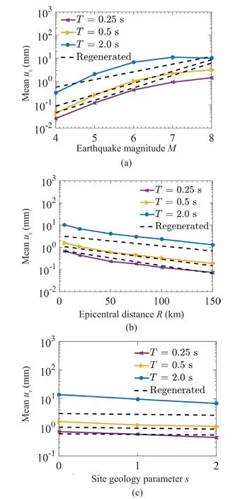
Fig.12 Comparison of actual and regenerated variations of logarithm of mean residual displacement with(a) earthquake magnitude M, (b) epicentral distance R,and (c) site geology parameter s at different periods for the bilinear model with μ = 4, αh = 0.1, αc = -0.1,δc/δy = 2, γ = 100

For a fixed set of periodTand model parameters(μin the case of the bilinear model, andμandkd,fin the case of the pinching model), the residual errors are computed for all 239ur(T) values by using this equation,and the actual probability distributionp*(ε(T)) is determined from the fractions of these residual errors.This probability distribution may be approximated by a Gaussian distribution with the meanm(T) and standard deviationσ(T), which is described as:

Fig.13 Comparison of actual and regenerated variations of logarithm of mean residual displacement with (a) earthquake magnitude M, (b) epicentral distance R, and (c) site geology parameter s at different periods for the pinching model with μ = 4, αh = 0.1,αc = -0.1, δc/δy = 2, γ = 100 and kd,f = 0.5

Fig.14 Comparison of actual and regenerated variations of logarithm of mean residual displacement with (a) post-yield stiffness ratio αh, (b) post-capping stiffness ratio αc, and (c) peak to yield displacement ratio δc/δy, of the bilinear model at different periods under ground motions with M = 6, R = 20 km, H = 5 km, s = 2

Fig.15 Comparison of actual and regenerated variations of logarithm of mean residual displacement with (a) post-yield stiffness ratio αh, (b) post-capping stiffness ratio αc, and (c) peak to yield displacement ratio δc/δy, of the pinching model at different periods under ground motions with M = 6, R = 20 km, H = 5 km, s = 2

The values ofm(T) =mˆ(T) andσ(T) =σˆ(T), which provide the best fit ofp(ε(T)) withp*(ε(T)), are estimated for different values of periodT; next, they are smoothed alongT.The smoothed values ofmˆ(T)andσˆ(T) corresponding to the regression coefficient estimates listed in Tables S6-S17 are provided in those tables for 17 selected periods.

The smoothed values ofmˆ(T) andσˆ(T) are used to estimate theε(T) values for the 46 periods considered forp= 0.1, 0.3, 0.5, 0.7, and 0.9.The so-obtained“estimated” error spectra are compared with the actual error spectra obtained forp*= 0.1, 0.3, 0.5, 0.7, and 0.9 in each of the 12 cases of bilinear and pinching models.The two sets of spectra are shown for the bilinear model withμ= 3, 4, 5 in Figs.16(a)-16(c), respectively.In the case of the pinching model withkd,f= 0.5, Figs.17(a)-17(c) show these spectra forμ= 3, 4, 5, respectively.For the cases of the pinching model withkd,f= 0.25 and 0.75, such spectra are displayed in Figs.S2 and S3 in Supplementary Materials.In each of these figures the actual spectra are shown by the use of solid lines and the estimated spectra are indicated by the dashed lines.These figures suggest that the actual error spectra are closely approximated by the estimated error spectra.The smoothed values ofmˆ(T) andσˆ(T) may be used to estimateε(T) for a given confidence levelpby using Eq.(5), which is then added to log10(T) obtained from Eq.(3) to lead to the residual displacement spectrum for confidence levelp(for a givenμin the case of the bilinear model, and a given set ofμandkd,fin the case of the pinching model).

Fig.16 Comparison of actual and estimated residual error spectra for different values of p = p＊ for the bilinear model with γ = 100 and (a) μ = 3, (b) μ = 4, (c) μ = 5

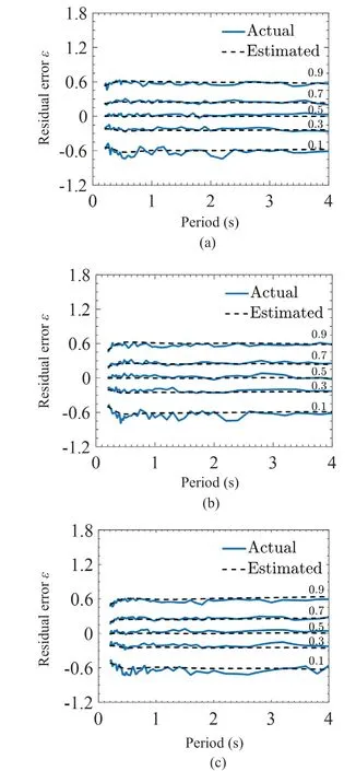
Fig.17 Comparison of actual and estimated residual error spectra for different values of p = p＊ for the pinching model with kd,f = 0.5, γ = 100 and (a) μ = 3, (b) μ = 4,(c) μ = 5

Two statistical “goodness of fit” tests, namely, the chi-square and Kolmogorov-Smirnov (KS) tests, are carried out to check the accuracy of the assumption ofp*(ε(T)) as the Gaussian distributionp(ε(T)), withm(T) andσ(T) taken as the smoothed values ofmˆ(T)andσˆ(T).The KS statistic KS(T) and the chi-square statisticχ2(T) are calculated for all 46 periods for a given set ofmˆ(T) andσˆ(T) and compared with the corresponding 95% cut-offlevels.Figures 18(a)-18(c)show these comparisons in the case of the chi-square test for the bilinear model havingμ= 3, 4, and 5,respectively.Figures 19(a)-19(c) show the comparisons in the case of the chi-square test for the pinching model withkd,f= 0.5 havingμ= 3, 4, 5, respectively.For the cases of the pinching model withkd,f= 0.25 and 0.75,such comparisons are shown in Figs.S4 and S5 in Supplementary Materials.Further, Figs.20(a)-20(c)show the comparisons of KS statistic KS(T) for the 46 periods with 95% cut-offlevels for the bilinear model,havingμ= 3, 4, and 5, respectively.Figures 21(a)-21(c) show such comparisons in the case of the pinching model withkd,f= 0.5, havingμ= 3, 4, 5, respectively.The comparisons for the cases of the pinching model withkd,f= 0.25 and 0.75 may be seen in Figs.S6 and S7 in Supplementary Materials.In each of these figures the statistical values are indicated by the filled circles and the cut-offlevels are specified by the dashed lines.It may be observed from these figures that both chi-square and KS statistics fall below the respective 95% cut-offlevels for most periods.There are 4 of 138 cases (thus a 2.9% probability) where the chi-square test fails in the case of the bilinear model.Further, there are 44 of 414 cases (thus a 10.6% probability) in which the chisquare test fails for the pinching model.Regarding the KS test, there are no cases in which the test fails in the case of the bilinear model, and there are 2 of 414 cases(thus a 0.5% probability) in which the test fails for the pinching model.Hence, even though there is a greater acceptability of the normal distribution as proposed (for the errors under the proposed scaling model for residual displacements) under the KS test and in the case of the bilinear model (compared to the pinching model), the assumption of normal distribution as in Eq.(5) may be considered acceptable for both the bilinear and pinching models.

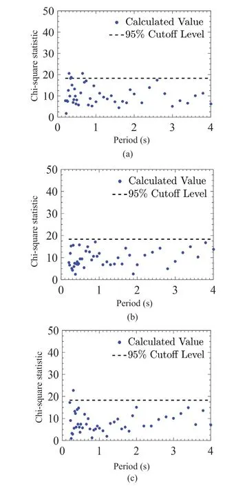
Fig.18 Comparison of chi-square statistics with a 95% cut-offlevel for different periods for the bilinear model with γ = 100 and (a) μ = 3, (b) μ = 4, (c) μ = 5

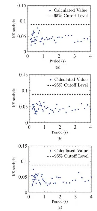
Fig.20 Comparison of KS statistics with 95% cut-offlevel at different periods for the bilinear model with γ = 100 and (a) μ = 3, (b) μ = 4, (c) μ = 5

It may be notable to learn how the mean (constantductility) residual displacement spectra predicted by the proposed scaling models (for bilinear and pinching oscillators) for different levels of confidence compare with theurspectrum obtained for a recorded ground motion.For this purpose, four ground motions are arbitrarily chosen from the suite of 1,076 motions considered above, and the residual displacement spectrumur(T) is calculated for each of these ground motions, while considering arbitrarily selected model parameters for each case.These spectra are then compared with the predicted spectra (by using the same values ofM,R, andsas for the recorded ground motion) forp= 0.1, 0.5, and 0.9.The chosen ground motions are (a) the S64E component of the 1957 San Francisco earthquake, recorded in the basement of City Hall, Oakland site, withM= 5.7,R= 39.9 km, ands=0; (b) the S00W component of the 1971 San Francisco earthquake, recorded in the basement at 2600 Nutwood Avenue, Fullerton site, withM= 6.4,R= 37.1 km, ands= 0; (c) the N45E component of the 1983 Coalinga earthquake, recorded at the Slack Canyon site, withM=6.5,R= 36.8 km, ands= 2; and (d) the N50W component of the 1994 Northridge earthquake, recorded at the 7420 Jaboneria Bell Gardens site, withM= 6.7,R= 48.5 km,ands= 0.The corresponding model parameters are (a)αh= 0.05,αc= -0.12,δc/δy= 3.61, (b)αh= 0.15,αc= -0.05,δc/δy= 2.02, (c)αh= 0.28,αc= -0.25,δc/δy= 2.95, and(d)αh= 0.22,αc= -0.1,δc/δy= 1.75.Other model parameters are taken uniformly asγ= 100,kd,f= 0.5, andμ= 4, with an initial damping ratio = 5%.Figures 22(a)-22(d) and 23(a)-23(d) respectively show the comparisons of actual and estimated spectra (forp= 0.1, 0.5, 0.9) for the bilinear and pinching models in the case of these ground motions.The actual spectra are shown by solid lines and estimated spectra are indicated by dashed lines in all of these figures.It may be observed in these figures that the 80%-confidence region bounded by the curves forp= 0.1 and 0.9 is very wide due to large variations in the response of bilinear and pinching oscillators with respect to different temporal characteristics of ground motions.However, most of the actual residual displacements in a figure lie within the 80%-confidence region and an almost equal number of displacements lie on both sides of the estimated spectrum forp= 0.5.Thus, the proposed scaling model can be considered as a reasonable model for predicting residual displacement spectra, while also accounting for uncertainties in the residual displacement response of a bilinear or pinching oscillator to the temporal characteristics of a given ground motion, besides the inherent uncertainties in the temporal characteristics of an anticipated ground motion.

Fig.21 Comparison of KS statistics with 95% cut-offlevel at different periods for the pinching model with kd,f = 0.5, γ = 100 and (a) μ = 3, (b) μ = 4, (c) μ = 5

Fig.22 Comparison of actual and estimated residual displacement spectra for different levels of confidence in the case of the bilinear model with μ = 4, γ = 100,and (a) αh = 0.05, αc = -0.12, δc/δy = 3.16; (b) αh = 0.15,αc = -0.05, δc/δy = 2.02; (c) αh = 0.28, αc = -0.25, δc/δy = 2.95;(d) αh= 0.22, αc = -0.1, δc/δy = 1.75; under (a) 1957 San Francisco, (b) 1971 San Francisco, (c) 1983 Coalinga,and (d) 1994 Northridge motions

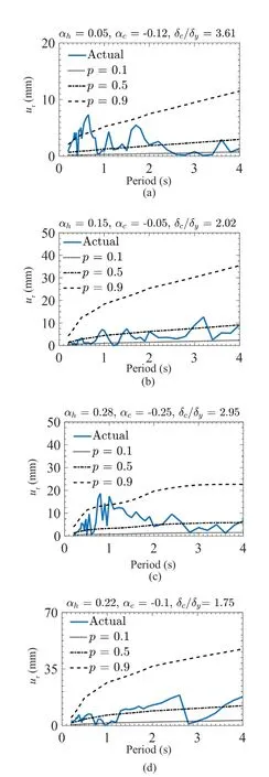
Fig.23 Comparison of actual and estimated residual displacement spectra for different levels of confidence in the case of the pinching model with μ = 4, γ = 100,kd,f = 0.5 and (a) αh = 0.05, αc = -0.12, δc/δy = 3.61;(b) αh = 0.15, αc = -0.05, δc/δy = 2.02; (c) αh = 0.28, αc = -0.25,δc/δy = 2.95; (d) αh = 0.22, αc = -0.1, δc/δy = 1.75; under(a) 1957 San Francisco, (b) 1971 San Francisco, (c) 1983 Coalinga, and (d) 1994 Northridge motions

6 Parametric study on ur(T) spectrum

The proposed scaling model is used to illustrate how theurspectrum for a given level of confidence changes with respect to each of the governing parameters that are considered, with the other governing parameters being held constant.The median residual displacement spectrum (corresponding top= 0.5) is considered for this purpose, with the seismological, site and model parameters taken the same as in the base case, i.e.,M=6,R= 20 km,s= 2,αh= 0.1,αc= -0.1 ,δc/δy= 2,γ=100,kd,f= 0.5,μ= 4, and with an initial damping ratio =5%.Figures 24(a)-24(c) and 25(a)-25(c) show the estimatedurspectra in the case of bilinear and pinching oscillators, respectively, when only the parametric variations with respect to earthquake magnitudeM,epicentral distanceR, and geological site condition parametersare considered.Figures 26(a)-26(d) and 27(a)-27(e) show the estimatedurspectra in the case of bilinear and pinching oscillators, respectively, when only the parametric variations with respect to post-yield strain hardening ratioαh, post-capping stiffness ratioαc, peak displacement to yield displacement ratioδc/δy,ductility ratioμ, and the pinching parameterskd=kf(for the pinching model) are considered.While all the curves predicted by the proposed scaling model show monotonically increasing residual displacements with an increase in oscillator period (with the other governing parameters held constant), some observations may be made regarding how the different governing parameters affect the residual displacement spectra for a given confidence level.

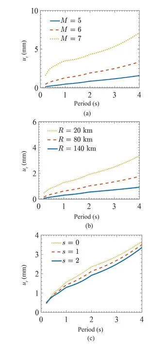
Fig.24 Estimated median residual displacement spectra for the bilinear model with μ = 4, αh = 0.1, αc = -0.1, δc/δy = 2 and γ = 100 under ground motions with different values of (a) earthquake magnitude M, (b) epicentral distance R, and (c) site geology parameter s

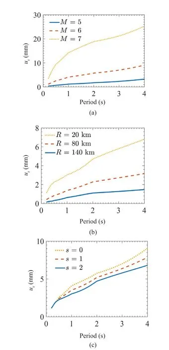
Fig.25 Estimated median residual displacement spectra for the bilinear model with μ = 4, αh= 0.1, αc = -0.1, δc/δy = 2,γ = 100 and kd,f = 0.5 under ground motions with different values of (a) earthquake magnitude M,(b) epicentral distance R, and (c) site geology parameter s

The effect of earthquake magnitude is that it increases the residual displacements for all periods, as seen from the curves shown forM= 5, 6, 7 in Figs.24(a)and 25(a).This increase is significantly higher as one moves fromM= 6 toM= 7, particularly in the case of the pinching model.However, a greater increase at higher magnitudes may be because the proposed scaling model does not capture the saturation in residual displacements with increasing earthquake magnitude.The effect of epicentral distance, as shown in Figs.24(b)and 25(b) through the curves forR= 20, 80, 140 km,is to increase the residual displacements for all periods with a decrease in the epicentral distance.Here again,this increase is significantly higher for smaller epicentral distances, particularly in the case of the pinching model,because the proposed model does not capture saturation in residual displacements with decreasing epicentral distance.Figures 24(c) and 25(c) show the effect of geological site condition; it may be observed that except for short periods, where this effect is insignificant, the alluvium conditions are associated with greater residual displacements for all periods.The increase appears to be within 30% in all the cases shown, as one moves from rock site conditions to alluvium site conditions.

The effect of the post-yield strain hardening ratioαhshown in Figs.26(a) and 27(a) (by means of the curves forαh= 0.01, 0.1, 0.2) is that the residual displacements for all periods are increased with a decrease in this ratio.This effect is, however, very pronounced in the case of bilinear oscillators and much smaller in the case of pinching oscillators.Further, there is a tendency of the residual displacements to saturate with increasing periods, particularly in the case of the pinching model.The negative effect of post-capping stiffness ratioαcis not so pronounced in the case of the bilinear model, as shown by the curves forαc= -0.01, -0.1, -0.2 in Fig.26(b).This effect is, however, slightly more (compared to that ofαh) in the case of the pinching model, as shown in Fig.27(b).The tendency of residual displacements to saturate at longer periods is observed here as in the case ofαh.Figures 26(c) and 27(c) display theurspectra forδc/δy= 2, 3, 4 in the case of bilinear and pinching models,respectively.It is clear from these figures that a higher value of peak displacement to yield displacement ratio(δc/δy) is associated with smaller residual displacements for all the periods and that this effect ofδc/δyis quite significant for both bilinear and pinching oscillators.Further, this effect ofδc/δyis more pronounced for the smaller values of this parameter.However, there is a tendency for the residual displacements to saturate with increasing periods in the case of the bilinear model.The residual displacements also rise significantly when the ductility ratioμincreases (for all periods), as shown by the spectra displayed in Figs.26(d) and 27(d) forμ= 3, 4,5.This rise, however, may be marginal for low-ductility bilinear oscillators.Finally, theurspectra shown in Fig.27(e) forkd,f= 0.25, 0.5, 0.75 demonstrate that even though the higher values ofkd,flead to smaller residual displacements, the variations in this parameter may not make much difference to the residual displacements of the pinching oscillators.

It may be mentioned that the observations made above may not hold in case any of the governing parameters other than the parameter being varied is not kept constant.For example, for a given set ofM,R, andsvalues, the inferences drawn regarding the role of peak displacement to yield displacement ratioδc/δyin the values of residual displacements may not hold if the ductility ratioμis not maintained.For the same reason, the actual spectra shown in Figs.22 and 23 reveal different trends compared to the estimated spectra, as oscillator periodTis varied, because each of the actual spectra shown conforms to different values ofpfor different periods.

Fig.26 Estimated median residual displacement spectra for the bilinear model with different values of (a) post-yield stiffness ratio αh, (b) post-capping stiffness ratio αc,(c) peak to yield displacement ratio δc/δy, and(d) ductility ratio μ under ground motions with M = 6,R = 20 km, and s = 2

Fig.27 Estimated median residual displacement spectra for the pinching model with different values of (a) post-yield stiffness ratio αh, (b) post-capping stiffness ratio αc,(c) peak to yield displacement ratio δc/δy, (d) ductility ratio μ, and (e) pinching parameters kd,f under ground motions with M = 6, R = 20 km, and s = 2

7 Summary and conclusions

A statistical estimation of a residual displacement spectrum has been attempted in the case of steel,reinforced concrete, and wood structures with hysteretic behaviors described by the bilinear and pinching models proposed by Ibarraet al.(2005).The bilinear model is described using four parameters, while the pinching model is described by the use of six parameters, for a given period, ductility demand, and initial damping ratio of the oscillator.

(a) A predictive model has been developed for a situation in which the seismic hazard at a site has not been characterized in the form of design spectra.The proposed model is based on a study on whether and how the residual displacement spectra that were averaged over an ensemble of spectrum-compatible ground motions depend upon various seismological, site, and model parameters.

(b) It has been found that for a given ductility ratio,initial damping ratio, oscillator period, and pinching parameterskdandkf(in the case of the pinching model),the logarithm of mean residual displacement depends almost linearly on earthquake magnitude (＜ 7), epicentral distance (＞ 20 km), site geology parameter, and model parameters, namely post-yield strain hardening ratioαh,post-capping stiffness ratioαc, and peak displacement to yield displacement ratioδc/δy.

(c) The dependence upon the hysteretic energy capacity coefficientγhas been found to be negligible,and no consistent trends have been observed as regards the dependence upon strong-motion duration.

(d) The (period-dependent) errors in the logarithm of the “best-fit” residual displacement spectrum have been assumed to follow a normal distribution, and the chi-square and Kolmogorov-Smirnov tests were carried out to validate this assumption.

(e) The proposed scaling model has been illustrated through the comparison of the predicted spectra for different levels of confidence with the actual spectra in the case of a few recorded motions.

(f) A parametric study carried out with the assistance of the proposed model shows how the variations in the mean residual displacement spectrum with respect to the parameters considered in the scaling model (i.e., earthquake magnitude, epicentral distance,site geology parameter, and model parametersαh,αc,andδc/δy) change with the oscillator period.This study also confirms that the median residual displacement spectra have greater amplitudes for all periods for higher ductility ratios in both the bilinear and pinching models.

(g) In the case of pinching oscillators, higher values of pinching parameters, when those are considered to be equal, lead to slightly smaller median residual displacements.

It should be mentioned that the proposed direct model is only a preliminary model, as this considers basic seismological parameters and is not applicable to earthquake magnitudes higher than 7 and/or epicentral distances less than 20 km.Further, this model may not be applicable to seismic regions that have different characteristics than those observed in the western U.S.region.

Electronic Supplementary Material: Supplementary material is available in the online version of this article at https://doi.org/10.1007/s11803-023-2220-x