Evaluation of meteorological predictions by the WRF model at Barrow,Alaska and Summit,Greenland in the Arctic in April 2019

ZHANG Tong, CAO Le, LI Simeng & WANG Jiandong

Article

Evaluation of meteorological predictions by the WRF model at Barrow,Alaska and Summit,Greenland in the Arctic in April 2019

ZHANG Tong, CAO Le*, LI Simeng & WANG Jiandong

China Meteorological Administration Aerosol-Cloud-Precipitation Key Laboratory, Nanjing University of Information Science & Technology, Nanjing 210044, China

Accurate meteorological predictions in the Arctic are important in response to the rapid climate change and insufficient meteorological observations in the Arctic. In this study, we adopted a high-resolution Weather Research and Forecasting (WRF) model to simulate the meteorology at two Arctic stations (Barrow and Summit) in April 2019. Simulation results were also evaluated by using surface measurements and statistical parameters. In addition, weather charts during the studied time period were also used to assess the model performance. The results demonstrate that the WRF model is able to accurately capture the meteorological parameters for the two Arctic stations and the weather systems such as cyclones and anticyclones in the Arctic. Moreover, we found the model performance in predicting the surface pressure the best while the performance in predicting the wind the worst among these meteorological predictions. However, the wind predictions at these Arctic stations were found to be more accurate than those at urban stations in mid-latitude regions, due to the differences in land features and anthropogentic heat sources between these regions. In addition, a comparison of the simulation results showed that the prediction of meteorological conditions at Summit is superior to that at Barrow. Possible reasons for the deviations in temperature predictions between these two Arctic stations are uncertainties in the treatments of the sea ice and the cloud in the model. With respect to the wind, the deviations may source from the overestimation of the wind over the sea and at coastal stations.

Arctic, WRF, meteorological parameters, synoptic patterns, model assessment

1 Introduction

The Arctic is the northernmost region of the earth and is centered on the North Pole (Ingold et al., 2022). Scientists defined the Arctic as a region within a line of latitude around the Earth, about 66.5°N, known as the Arctic Circle. Regions within the Arctic Circle include the Arctic Ocean basin and some northern parts of Greenland, Scandinavia, Russia, Canada, and the US. The climate of Arctic regions varies greatly, depending on their latitude, proximity of the sea, elevation and topography, but, even so, they all share certain “polar” characteristics. As we know, the Arctic is cold all year round and is largely covered by water. Most of the water covering the Arctic is frozen throughout the year, which includes sea ice floating in the sea, land ice (i.e., glaciers and ice sheets), icebergs, snow and permafrost. And due to the extreme solar radiation experienced in the high latitudes, the Arctic has at least one 24-hour period in each winter when the sun does not rise and the sea is largely frozen. Similarly, there is at least one 24-hour period in each summer when the sun does not set and the sea ice margins of the Arctic Ocean melt. The length of the continuous day or night increases northward, from 1 d at the Arctic Circle to 6 months at the North Pole.

The climate of the Arctic region has undergone a significant alteration in recent decades. A report titled “Arctic Climate Change Update 2021: Key Trends and Impact” was published by the Arctic Monitoring and Assessment Program (AMAP) of the Arctic Council in May 2021 (AMAP, 2021). According to this report, the near-surface Arctic temperature has increased by 3.1 ℃ over the past 49 years (1971–2019), which is roughly three times the global average. This significant temperature increase in the Arctic has had a substantial impact on the region’s precipitation, sea ice, land ice, permafrost, snowpack, and glacier melting. Additionally, the frequency of localized extreme events (e.g., extreme cyclones, high heat, excessive melt, rapid ice loss, and extreme wind) in the Arctic is rising. According to previous studies (Holland et al., 2006; Bhatt et al., 2014), the Arctic Ocean will be completely ice-free for the first time in September 2040. Furthermore, they speculated that by 2050, there may be no summer sea ice in the Arctic.

Climate change in the Arctic has a tremendous impact on not only the ecosystems but also the human lives and the transportation in this region. Additionally, there is a direct connection between severe weathers in mid-latitudes and the climate change in the Arctic. Consequently, it is crucial to accurately capture the meteorological changes in the Arctic. However, compared to the mid- and low-latitudes, the Arctic has fewer automatic weather stations due to the harsher environmental conditions. Additionally, the COVID-19 outbreak also affected recent Arctic observations, causing gaps in the 2020–2021 measurements. As a result, numerous Arctic research programs and initiatives have been delayed due to the lack of meteorological observations (AMAP, 2021). Thus, meteorological simulations are considered to be crucial complements to meteorological observations in the Arctic.

Previous scholars have made many efforts and advancements in simulating Arctic meteorological conditions. Bromwich et al. (2001), for example, employed Polar MM5 for mesoscale simulations of kabatatic winds across Greenland in the Arctic. Polar MM5 can simulate both large-scale and low-level atmospheric phenomena over the Greenland Ice Sheet, according to the simulation results. Cassano et al. (2001) also employed Polar MM5 to successfully predict the Greenland atmospheric circulation over a 48-hour period in all seasons. Afterwards, WRF has gradually been used as a replacement for the Polar MM5. Since its first release, the WRF model performance in polar applications has been assessed by the polar atmospheric modeling community (Cassano et al., 2011). For example, researches such as that conducted by Hines and Bromwich (2008) and Bromwich et al. (2009) indicated that WRF has equivalent or greater skills in simulating the atmospheric situations over Greenland and the Arctic Ocean compared to Polar MM5. Besides, Dong et al. (2018) used the WRF model to investigate surface wind characteristics in high-latitude regions, and the model was found to perform well in reproducing high-latitude strong winds when the roughness length was carefully given while taking vegetation type into account.

However, simulations of meteorological conditions in the Arctic are still insufficient. At present, numerical studies of meteorological parameters have mostly been conducted for mid and low latitude regions (Tse et al., 2014). Also, relevant studies in the Arctic were mostly carried out in coarse spatial resolutions. Besides, they usually focused on a single station or area. In contrast, to tackle deficiencies for meteorological predictions, a high horizontal spatial resolution in numerical models should be used and simulated results should be validated by using measure- ments from multiple stations. Therefore, in this study, we used a recent version of WRF and set a high grid resolution (3 km) to numerically simulate the meteoro-logical conditions at two Arctic stations (BRW and SUM) and the surroundings in April 2019. And the results showed that the three-dimensional high-resolution numerical model is capable of reproducing the observed meteorological features, exhibiting high correlation coefficients and small deviations.

In Section 2 of this paper, we show the studied area and data sources, describe the configurations of WRF model and statistical parameters, and introduce the methods to analyze synoptic patterns. In Section 3, we evaluate WRF model performance in simulating meteorological parameters and weather systems in the Arctic. Additionally, we also compare the results between the two stations investigated in this study and identify possible causes of deviations in the simulation results. At last, in Section 4, we list the key conclusions and suggestions for further research.

2 Methodologies

2.1 Monitoring stations and observational data

In this study, we chose two monitoring stations, Barrow Atmospheric Baseline Observatory (BRW) and Summit Atmospheric Baseline Observatory (SUM) to investigate (Figure 1).

The BRW station (71.3230°N, 156.6114°W, 8 m above sea level), built in 1973, is located on the northmost point of the US. It is located about 8 km northeast of the village of Utqiaġvik (formerly known as Barrow), Alaska. And it has a predominant east-northeast wind off the Beaufort Sea. At BRW, routine examination and maintenance of instruments are performed at least 5 d for a week. Although the measurements at BRW are conducted over open tundra, the Arctic Ocean is located less than 3 km to the northwest of the station, and there are numerous lakes and large lagoons nearby. As a result, BRW is appropriately described as having an Arctic maritime climate that is influenced by changes in weather and sea ice conditions in the Central Arctic.

Figure 1 The geographical locations of two stations (i.e., BRW and SUM) investigated in this study.

In contrast, the SUM station (72.6°N, 38.4167°W, more than 3200 m above sea level) is located on the center of the Greenland Ice Sheet (Showstack, 2011). The SUM station on the summit of the Greenland Ice Sheet was jointly established by the US National Science Foundation (NSF) and National Oceanic and Atmospheric Administration (NOAA) with the permission of the Danish Commission for Scientific Research in Greenland to provide year-round, long-term measurements for monitoring and investigating the Arctic environment. The SUM station is equipped with surface ozone monitoring instrumentation, a basic meteorology system, aerosol instrumentation, and greenhouse and halocarbon gas flask sampling capabilities. And it is in partnership with the NSF to best meet NOAA’s mission and the nation’s scientific needs. The topography in SUM is flat and uniform, with mostly gently downward sloping terrain surrounding this station (Helmig et al., 2007).

The BRW and SUM meteorological measurements were taken from Earth System Research Laboratory (ESRL) /Global Monitoring Division (GMD) Baseline Observatorieswebsite of NOAA (https://gml.noaa.gov/aftp/data/meteorology/ insitu/), which are freely provided to the public and the scientific community. The data used in this study include surface pressure, temperature at 2 m, wind speed and wind direction at 10 m, with a time resolution of 1 h from 1 April to 1 May, 2019 (UTC).

2.2 WRF model configurations

In this study, we adopted the WRF model (Skamarock et al., 2019), a three-dimensional atmospheric modeling system, to capture the change of meteorological parameters in the Arctic. The WRF model was developed through a partnership of the National Center for Atmospheric Research (NCAR), NOAA (represented by the National Centers for Environmental Prediction (NCEP) and NOAA ESRL), the US Air Force, the Naval Research Laboratory, University of Oklahoma, and the Federal Aviation Administration. In this study, we used WRF version 4.2.2, with an Advanced Research WRF (ARW) dynamical solver. The ARW solver is a flexible, state-of-the-art atmospheric simulation system that is portable and efficient on available parallel computing platforms.

The WRF model was set to run for the entire April of 2019 for two stations (i.e., BRW and SUM). In the Arctic region, many special atmospheric phenomena such as the stratospheric ozone holes (Manney et al., 2011; Alwarda et al., 2021) and the tropospheric ozone depletion events (Herrmann et al., 2021; Cao et al., 2023) occur in the springtime. During these phenomena, meteorological conditions are extremely important for the occurrence and termination of these events. Moreover, daily variations of surface meteorological parameters are more significant in the Arctic spring. In addition, our available computational resources can only support one-month simulations due to limitations. Thus, April 2019 was chosen as the representative month for evaluating the WRF performance in this study. The polar stereo-graphic projection was used. The model ran continuously 30 d in total with the first 2 d taken as a spin-up time. Two nested areas (d01 and d02) were used for the simulations of BRW and SUM (Figure 2). In these two nested areas, 367 east-west and 321 north- south grid cells were distributed in d01, covering a 3294 × 3880 km2area. The d02 has 370 east-west and 322 north- south grid cells covering a 1107 × 963 km2area. Along the vertical direction, 35 layers were set from the ground to the top pressure of 50 hPa, and time step is 45 s in d01 and 15 s in d02. The Final Operational Global Analysis (FNL) dataset (NCEP et al., 2000) ranging from 1 April to 1 May, 2019 (UTC), with 1°× 1° grid resolution every 6 h, was used as the initial and boundary conditions of the WRF model. The model inputs of static geographical data, including terrain altitude, land use, land cover, soil type, albedo and leaf area index, were adopted from the Moderate Resolution Imaging Spectroradiometer (MODIS) data (Friedl et al., 2002, 2010), with a horizontal grid resolution of approximately 1 km. Among these parameters, the land use and the soil type were classified into 21 and 16 categories, respectively. Aside from that, the model inputs of soil temperature, soil moisture, snow temperature, snow depth and sea ice information were obtained via the FNL dataset (NCEP et al., 2000), with a spatial resolution of 1°× 1°.

Table 1 lists the WRF configurations and parameterizationschemes used in each simulation. Thompson scheme (Thompson et al., 2008) was used as the micro-physical scheme, and Mellor-Yamada-Janjić (MYJ) scheme (Mellor and Yamada, 1982) was used as the planetary boundary layer scheme. RRTMG, which refers to the Rapid Radiative Transfer Model for GCMs (global circulation models) (Iacono et al., 2008), was used as the shortwave and longwave radiation schemes, and Modifed Tiedtke scheme (Tiedtke, 1989; Zhang et al., 2011) was used as the cumulus convection scheme. Besides, Noah scheme (Niu et al., 2011) was used as the land-surface model, and Monin-Obukhov (Janjić Eta) scheme (Janjić, 1994) was used as the surface-layer model. In previous model studies (Wilson et al., 2011, 2012) investigating the surface and upper air features and the atmospheric hydrologic cycle over the Arctic, it has been proved that the Noah scheme and the Monin-Obukhov (Janjić Eta) scheme can accurately estimate the exchange of heat, momentum and moisture between the land surface and the atmosphere in the Arctic.

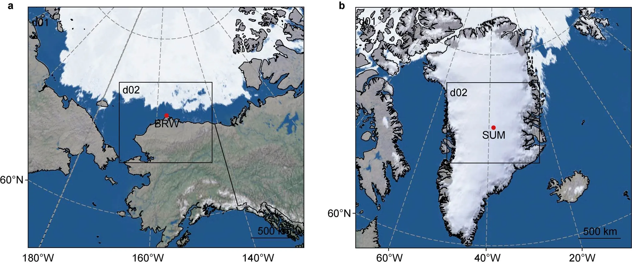
Figure 2 Computational areas for BRW (a) and SUM (b) simulations. The red points represent the locations of these two stations.

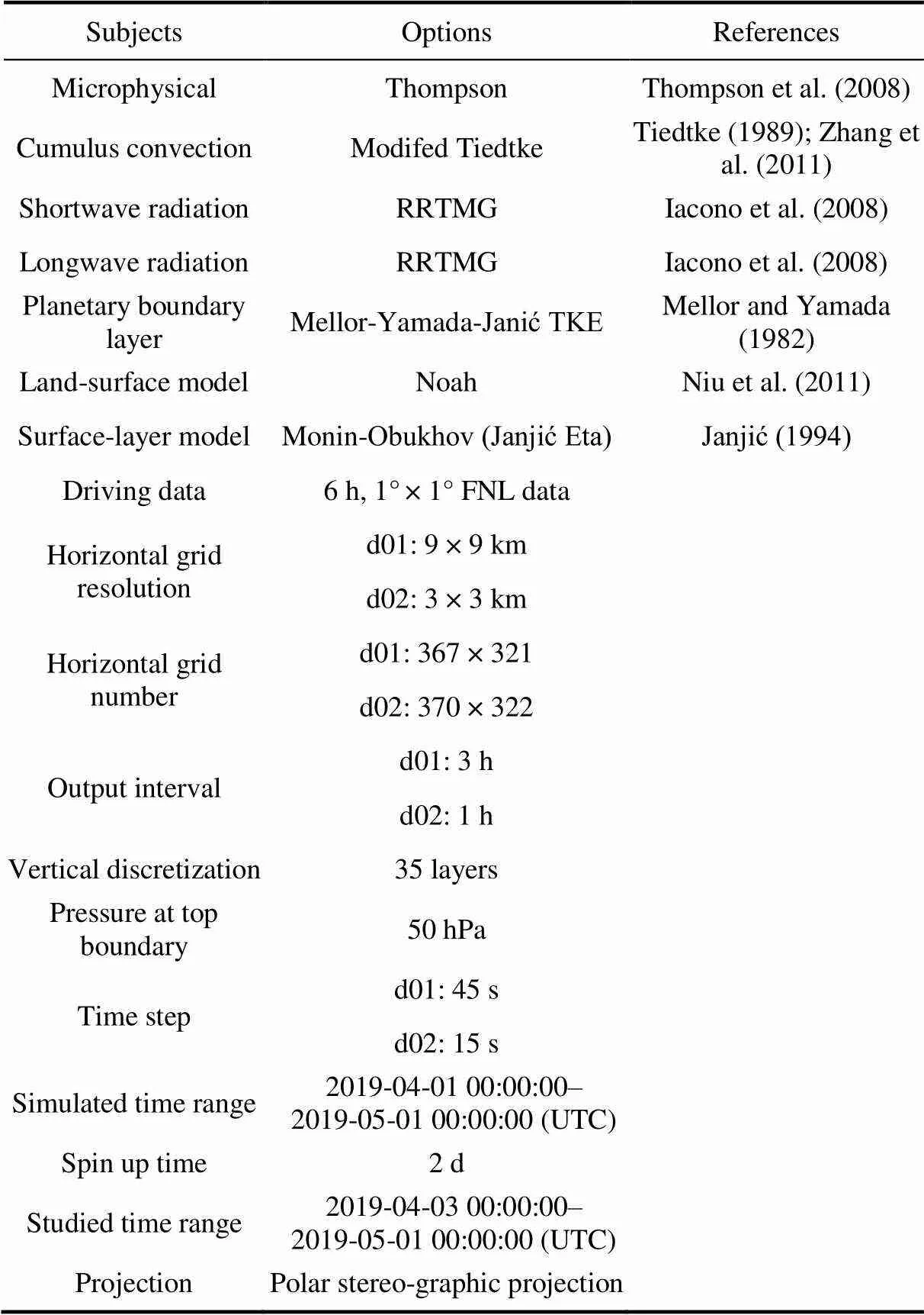
Table 1 Physical parameterization schemes and configurations used in WRF simulations

2.3 Statistical parameters for evaluating the model performance

In this study, we used five statistical parameters to evaluate the model performance, namely Pearson correlation coefficient (), index of agreement (IOA), root mean square error (RMSE), mean bias (MB) and mean absolute gross error (MAGE) (Zhang et al., 2012; Emery et al., 2017). These statistical metrics were used to quantitatively estimate the consistency between the measurements of meteorological parameters and the simulation results for BRW and SUM. Among these statistical parameters, Pearson correlation coefficient () is a linear correlation coefficient and is one of the most commonly used coefficients. It is defined as:

The IOA is calculated as follows:

IOA can also reflect the agreement between simulated and observed values. Different from, IOA not only depicts the consistency in the trend but also reflects the deviation between observations and simulations. The value of IOA is between 0 and 1, when a value of 1 indicates a perfect correlation.

RMSE is defined as shown in Equation (3):

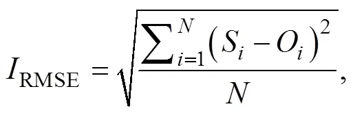
RMSE is the square root of the ratio of the square of the difference between the simulated and observed values to the observation times. It can be used to indicate the degree of fitting between simulations and observations, so as to measure the bias between simulations and observations. RMSE is sensitive to large or small errors in simulations, so RMSE can reflect the precision of simulations. Thus, RMSE equal to zero is associated with the best quality of simulations.

The calculation of MB is as follows:

MB is used to evaluate the data tendency and measure the bias between modelled values and observed values. A positive (negative) bias means the simulations overestimate (underestimate) the measured values.

MAGE shown in Equation (5), represents an average value of the absolute error between measurements and simulations:

(5)

2.4 Surface weather charts

Surface weather charts were used to find important weather systems with different scales, such as high/low pressure systems, troughs, ridges and fronts. Moreover, important weather systems showed in the weather charts were also compared with simulations to verify the model predictions.

The surface weather charts are provided by the Weather Prediction Center (WPC). WPC is one of nine centers of the NCEP and archives a selection of US and North American surface weather charts. These charts can depict the synoptic and sub-synoptic/mesoscale weather patterns including highs, lows, fronts, troughs, outflow boundaries, squall lines, and drylines. Available weather charts start from the year 2005 to present, and the time resolution is 3 h. The area included in these charts covers most of North America, the western Atlantic and eastern Pacific oceans, and the Gulf of Mexico. The BRW and SUM stations are also included in this area. In this study, we adopted the surface weather charts from 00:00 on 3 April to 21:00 on 30 April, 2019 (UTC) to analyze (Table 1).

3 Results and discussions

In this section, we quantitatively evaluate the model performance in capturing meteorological parameters at the BRW and SUM stations and analyze the changes in synoptic patterns in the focused regions during April 2019. Furthermore, we investigate possible reasons for deviations between simulations and observations.

3.1 Evaluation of one-month meteorological simulations at BRW and SUM

We first assessed the WRF model performance in simulating surface pressure, 2 m temperature, and horizontal components of wind speed at 10 m at the BRW and SUM stations from 00:00 on 3 April to 00:00 on 1 May, 2019 (UTC).

3.1.1 WRF results for surface pressure

Figure 3 provides a comparison of surface pressure () between simulated and observed values at BRW and SUM during the studied period. It can be seen in Figure 3a that during the analyzed time period, the surface pressure at BRW peaked at 00:00 on 3 April (UTC). After that, there was a sharp decrease for several days. Until 8 April, 2019, the surface pressure dropped by about 30 hPa. The surface pressure subsequently fluctuated over the rest of April, which may be related to the weather activities nearby. It is also seen in Figure 3a that the simulations of surface pressure by the WRF model are in good agreement with the observations, both in peak and trough values. Furthermore, Figure 3b shows that the largest difference between the simulated and observed values at the BRW station is less than 6 hPa, exhibiting small model deviations. The assessment parameters associated with the surface pressure at the BRW station listed in Table 2 also indicate that the simulations of surface pressure are credible during the studied period.

Likewise, as for SUM, it is shown in Figure 3c that the surface pressure rose continuously from 3 to 8 April, then fell gradually from 8 to 18 April. After that, the surface pressure remained relatively stable for the next few days, then began to increase on 24 April until reaching a maximum on 30 April. As shown in Figure 3c, the simulations of surface pressure at SUM are similar to observations, with high(0.99) and IOA (0.99). It is also presented in Figure 3d that most of the deviations are within ±2.5 hPa. The high accuracy in surface pressure simulations at SUM is also reflected by the small RMSE (1.65 hPa), MB (−1.13 hPa) and MAGE (1.34 hPa) (Table 2).

Figure 3 Time series of surface pressure obtained from simulations and observations for BRW (a) and SUM (c). Differences between simulations and observations are also presented in (b) and (d).

Table 2 Statistical assessments of the meteorological simulations at both stations

In general, the WRF model, at both stations, accurately captured the changes of surface pressure during the analyzed period. However, from the comparison of five statistical parameters between these two stations (Table 2), not onlyand IOA at SUM are greater than those at BRW, but also the deviations at SUM are less than those at BRW. Thus, the simulation of surface pressure at the SUM station is overall better than that at BRW.

3.1.2 WRF results for 2 m temperature

In Figure 4, it presents a comparison of 2 m temperature () between simulations and observations at two stations. It can be seen in Figure 4a that the observed 2 m temperature at BRW ranges from −27.1 ℃ to 2.8 ℃ in April, and it increases slowly as time goes by. The temperature at BRW has a relatively small diurnal variation due to the coastal marine environment of this station. Figure 4a shows that the simulations of 2 m temperature at BRW are similar to observations. The five statistical parameters (i.e.,, IOA, RMSE, MB and MAGE) are 0.79, 0.88, 3.75 ℃, −1.14 ℃ and 2.95 ℃, respectively (Table 2), indicating the simulated 2 m temperature at BRW consistent with the observations. It also shows in Figure 4b that the deviations in 2 m temperature at BRW are smaller than 10 ℃ in most of April. However, the diurnal variation of 2 m temperature in simulations was found to be greater than that in observations. Moreover, most of the simulated values are lower than observed values during the studied period, especially from 14 to 20 April. Thus, there is an overall negative bias in model simulations at BRW (MB = −1.14 ℃).

Figure 4c displays the time series of temperature at 2 m obtained from simulations and observation at SUM in April. The 2 m observed temperature at SUM ranges from −44.9 ℃ to −9.4 ℃, with wide fluctuations in the diurnal variation. At SUM, the simulated 2 m temperature exhibits a strong correlation with the measurements (= 0.86, IOA = 0.92). The 2 m temperature difference at SUM is also less than 10 ℃ in most of time (Figure 4d). In addition, the simulated 2 m temperature at SUM has a low RMSE of 4.12 ℃ and MAGE of 3.25 ℃ (Table 2). Thus, the WRF model is able to reproduce the behavior of 2 m temperature at SUM, although the simulations slightly overestimated the observations (MB = 1.07 ℃).

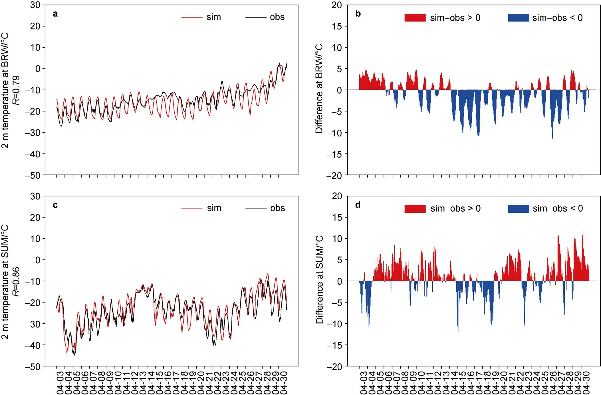
Figure 4 A comparison between simulations and observations for 2 m temperature at BRW (a) and SUM (c). Differences between simulations and observations are also presented in (b) and (d).

From the comparison of Figure 4a and Figure 4c, it can been seen that the 2 m temperature at SUM is mostly lower than that at BRW during April, due to the high altitude of SUM (more than 3000 m). Diurnal variation of temperature at SUM was also found to be stronger than that at BRW. It is because the BRW station is a coastal station, so that its atmosphere contains abundant water vapor and sea salt aerosols originated from the sea. The water vapor and aerosols in the atmosphere will absorb the longwave radiation emitted from the surface at night, which plays a role in thermal insulation, thus increasing the daily minimum temperature (Sokolowsky et al., 2020). Furthermore, the large amount of water vapor and aerosols in the atmosphere of BRW would facilitate the formation of clouds, which may reduce the solar radiation reaching the ground surface during the daytime, leading to a lower daily maximum temperature, and also increase the minimum daily temperature by enhancing downward longwave radiation during the nighttime (Pyrgou et al., 2019). Therefore, the diurnal variation of temperature at BRW is small. In contrast, SUM is a high-altitude land station with thin air and low water vapor concentrations. As a result, the total solar radiation reaching the ground surface is strong during the daytime, which heats up the surface quickly. Moreover, the ground surface cools down rapidly at night because the longwave radiation released by the surface can penetrate the thin dry air more easily. Thus, SUM has a relatively strong diurnal temperature variation.

From assessment parameters of these two stations, it was found that the 2 m temperature simulations at SUM are in better agreement compared with those at BRW. The major deviation in BRW temperature simulation was sourced from the temperature underestimation during 14–21 April. We found that during this time period, a high-pressure center was situated to the northeast of the BRW station on 14 April (see H1 in Figure S1a). Then, between 14 and 16 April, another anticyclone (H2 in Figure S1b) also started to form in the Arctic Ocean, and moved towards the BRW station. This intense anticyclone stayed in the Beaufort Sea to the northwest of BRW until 21 April (see Figures S1c and S1d). As a result, under the influence of anticyclones H1 and H2, the BRW station was dominated by northerly winds that carried marine air originated from the Beaufort Sea during 14–21 April.

In previous studies using different models (Lucas-Picher et al., 2012; Zhang et al., 2022), an underestimation of temperature at coastal stations in the Arctic was also reported. It was suggested that in present models, constant values are mostly adopted for sea ice parameters so that the changes in sea ice cannot be accurately represented (Hines et al., 2015; Zhang et al., 2022), leading to the uncertainty in temperature simulations at coastal stations. Besides, the spatial resolution of our sea-ice data (1° × 1°) is still low compared to the grid resolution of the WRF model (3 km × 3 km), which might be another a reason contributing to the deviations.

In addition, the WRF model currently provides a variety of cumulus parameterization schemes, and the simulation effects of choosing different parameter- zation schemes vary significantly for different regions and atmospheric phenomena. Therefore, another possible reason is that the cloud is not adequately considered in the present model, so that the interaction between the cloud and the radiation is not precisely parameterized (Bromwich et al., 2013; King et al., 2015). Zhang et al. (2011) used the WRF model coupled with the modified Tiedtke scheme to simulate the marine boundary layer clouds, but found discrepancies between simulations and observations. Thus, the modified Tiedtke scheme adopted in this study can also cause the deviations in cloud simulations for the BRW station, resulting in the temperature biases. Besides, the uncertainty in estimating the radiation may also cause the deviation in temperature simulations at these Arctic stations.

To sum up, the simulation results for 2 m temperature are credible at both stations, but the results at SUM are superior to those at BRW due to the uncertainties in the treatments of the sea ice and the cloud in the model.

3.1.3 WRF results for zonal and meridional winds

The WRF model also simulated the 10 m wind at both stations. In this study, the zonal wind () is represented by U-wind, and a value greater than zero indicates a westerly wind. Similarly, the meridional wind () is represented by V-wind, and a value greater than zero indicates a southerly wind. Observations of 10 m wind were also decomposed into zonal and meridional winds for comparison. A comparison between the simulated and observed winds at BRW is presented in Figures 5a and 5c. It is displayed that U-wind and V-wind at BRW are mostly negative during April, indicating a predominant northeasterly wind at the BRW station. Zonal and meridional wind speeds are from −11.86to 4.03 m·s–1and from −10.01 to 6.63 m·s–1. Differences between simulations and observations of zonal and meridional winds are less than 5 m·s–1in most of time (Figures 5b and 5d)., IOA, RMSE, MB and MAGE are 0.78, 0.88, 2.28 m·s–1, 0.51 m·s–1and 1.63 m·s–1for U-wind at BRW and 0.74, 0.83, 2.68 m·s–1, 1.24 m·s–1and 2.16 m·s–1for V-wind at BRW (Table 2). According to these statistical parameters, winds at BRW are predicted well with high correlations and small deviations.

Figures 5e and 5g present a comparison between simulated and observed winds at SUM. The prevailing wind at SUM is mainly southeastern and the wind speed is within 15 m·s–1. It is seen from Figures 5f and 5h that differences between simulations and observations are within 5 m·s–1in most of time. In addition, the five statistical metrics (i.e.,, IOA, RMSE, MB and MAGE) of U-wind are 0.88, 0.92, 2.09 m·s–1, 1.01 m·s–1and 1.66 m·s–1at SUM, respectively. And these assessment parameters of V-wind are 0.79, 0.86, 2.38 m·s–1, 1.14 m·s–1and 1.80 m·s–1, respectively (Table 2). It shows that the changes in wind at SUM can also be accurately captured.

Based on the statistical parameters of these meteorological variables shown in Table 2, we found the model performance in predicting the V-wind the worst at both stations, which deteriorates the predictions of the 10 m wind. As a result, our model shows comparatively less skills in simulating the 10 m wind as compared to other variables. It is because the wind is a highly dynamic variable that can be largely influenced by local factors such as topographical features. Kadaverugu et al. (2021) also suggested that dynamic variables (e.g., wind direction and wind speed) are less accurately predicted by the WRF model than thermodynamic variables (e.g., temperature), which is consistent with our results. Moreover, we found the performance of the WRF model in simulating the winds at these two Arctic stations better than that at other regions, especially mid-and low-latitude urban stations (Yang et al., 2012; Surussavadee, 2017; Kadaverugu et al., 2021; Solbakken et al., 2021), which might be caused by two reasons. The first reason is the differences in land features between Arctic stations and urban stations. BRW and SUM in the Arctic have a relatively flat and uniform topography, and are less influenced by the presence of buildings and vegetation. As a result, the winds at the Arctic stations can be more accurately captured by the WRF model with a horizontal resolution of several kilometers. In contrast, urban stations, with small-scale complex topography and multiple categories of underlying surfaces, have relatively large deviations in wind simulations. The second reason is the uncertainty in anthropogenic heat sources in the WRF model. The global population is predominantly distributed in mid-and low-latitude regions. Thus, wind predictions in the low-and mid-latitude regions by the WRF model were heavily affected by unspecified accounting of anthropogenic heat release in these regions (Zhan and Xie, 2022). In contrast, the smaller population and fewer heat sources in the Arctic may lead to a more accurate prediction of meteorological parameters at Arctic stations.

The comparison of statistical metrics between two stations demonstrates that the simulation of wind for BRW is inferior to that for SUM. As mentioned before, BRW is a coastal station and the prevailing wind during the studied period is mainly from the Beaufort Sea. We thus suggest that the deviations in U- and V-wind simulations at BRW may come from the overestimation of the wind speed over the Beaufort Sea. It is well known that surface properties such as the roughness length are key factors for near-surface wind predictions (Liu et al, 2022). However, the WRF model considers the sea as a flat surface with a constant height and roughness length, while the real sea has a larger roughness length because of the change in the height of the sea surface (Carvalho et al, 2013, 2014). The lower roughness length implemented in the model over the sea thus gives a higher wind prediction because of the smaller friction between the air and the sea surface. Hughes and Veron (2015) also obtained a conclusion that the simulating WRF bias of surface wind speed in coastal areas is larger than that in inland areas, which is in agreement with our results.

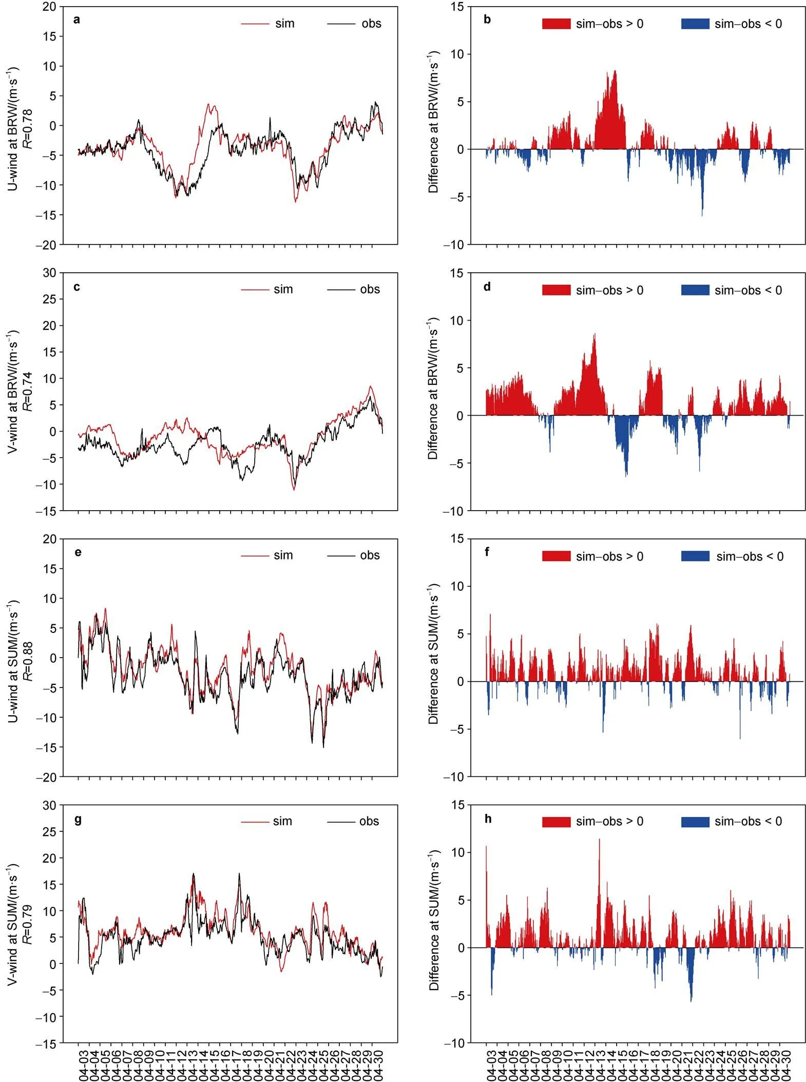
Figure 5 A comparison between simulations and observations for U-wind at BRW (a) and SUM (e), V-wind at BRW (c) and SUM (g). Differences between simulations and observations are also presented in U-wind (b) and V-wind (d) at BRW, and U-wind (f) and V-wind (h) at SUM.

The above results, containing surface pressure, 2 m temperature, zonal and meridional winds, reveal that WRF is capable of capturing meteorological parameters precisely in the Arctic during the studied period. Correlation coefficients for these meteorological parameters are generally above 0.74 throughout the entire month. Among these near-surface meteorological parameters, WRF predicts the surface pressure the best at both stations. In contrast, the prediction of the 10 m wind is the poorest among all these meteorological parameters. However, the wind simulations for these two Arctic stations were found to be much better compared with simulations for other regions such as mid- latitude regions. In addition, in our study, meteorological simulations for SUM are generally more accurate than those for BRW due to the differences in types of underlying surfaces (i.e., sea and land) and locations of the stations.

3.2 One-month synoptic analysis at BRW and SUM

An analysis of synoptic patterns in April, 2019 was performed in this study by using surface weather charts from WPC. The time resolution of the charts is 3 h. We selected 4 different time points (Figure 6) to analyze.

Figure 6 A selection of WPC surface weather charts (a–d) for the studied area. Different weather systems (i.e., cyclones and anticyclones) are marked using rectangles and their names are displayed in the top of the rectangles. Locations of the two Arctic stations (BRW and SUM) are also indicated using black points.

3.2.1 Synoptic analysis at BRW

The surface weather charts for the BRW station and surrounding areas are presented in Figure 6. It is seen in Figure 6a that a strong anticyclone (H1) appeared over the Beaufort Sea that is to the north of BRW on 3 April, and the high surface pressure at the center of the anticyclone reached 1042 hPa. At the same time, another anticyclone (H2) was also located over the Gulf of Alaska. Thus, the surface pressure at BRW was extremely high at this time, as shown in Figure 3a, because BRW was under the influence of these two high-pressure systems. Then, a new cyclonic system (L2 in Figure 6b) was gradually formed on the Gulf of Alaska, and thus BRW and nearby areas were later controlled by a low pressure, on 8 April as illustrated in Figure 6b. The surface pressure of BRW dropped to a minimal value at this time, which is consistent with the temporal change of surface pressure shown in Figure 3a. After that, due to continuously cyclonic and anticyclonic activities (L3, H4 in Figure 6c and L5, L6 in Figure 6d) formed on the Beaufort Sea and Gulf of Alaska, the surface pressure at BRW fluctuated, following the changes of weather systems in the rest of studied period.

3.2.2 Synoptic analysis at SUM

Figure 6 also shows the weather situations for the SUM station and surrounding areas. At first, a cyclonic system (L1 in Figure 6a) was formed in the southwestern coast of Greenland, accompanied by a low pressure center on 3 April. Thus, the surface pressure at SUM dropped, consistent with the results shown in Figure 3b. Then an anticyclone (H3 in Figure 6b) appeared in central Greenland, and thus SUM is then controlled by a high-pressure system. Next, the high pressure at Greenland was weakened and two intense cyclones (L4 in Figure 6c) were formed in the North Atlantic Ocean that is to the south of Greenland, and several low pressure centers (L7 and L8 in Figure 6d) also appeared near the SUM station on 15 April, so the surface pressure at SUM decreased gradually. Afterwards, SUM was consistently controlled by a high-pressure system, so the surface pressure gradually increased from 27 April to 30 April (Figure 3b).

3.2.3 Simulations of synoptic patterns at BRW and SUM

We displayed the spatial distributions of meteoro- logical parameters in WRF simulations during April (Figure 7 and Figure 8). The meteorological parameters included are sea level pressure, 2 m temperature, and 10 m wind. We compared the simulated weather systems (i.e., cyclones and anticyclones, low-pressure and high-pressure centers) surrounding both stations with those obtained from the weather analysis. We concluded that the locations of cyclones and anticyclones and the values of low-pressure and high-pressure centers in simulations are basically in good agreement with those shown in the weather charts. For example, it is seen in Figure 7a that the WRF model simulated an anticyclone (H1) over the Beaufort Sea, which is consistent with the surface weather chart shown in Figure 6a. Likewise, cyclones in western Greenland such as L1 shown in Figure 6a were also reproduced in Figure 8a. Thus, the WRF model is able to accurately capture the changes of synoptic patterns in the Arctic.

In summary, we found that cyclonic and anticyclonic systems occurred frequently in the Arctic during April 2019. These weather systems are major factors controlling the variation of meteorological parameters such as the pressure in the Arctic. Furthermore, the WRF model is able to accurately capture the changes of weather systems around these Arctic stations.

4 Conclusions

In the present study, we used the WRF model to simulate the meteorological changes in regions near two Arctic stations (i.e., BRW and SUM) during April 2019. The model performance in capturing meteorological parameters and weather systems is assessed and the reasons causing deviations between simulations and observations are also discussed.

Based on the comparison between WRF model simulations and observations, we found the model performance satisfying in capturing meteorological parameters in the Arctic. Among these meteorological parameters, the model was found to have the highest accuracy in predicting the surface pressure while it has the lowest accuracy in predicting the wind at these two Arctic stations. However, the wind predictions by the WRF model for the Arctic stations were found to be significantly better than that for urban stations in mid- or low-latitude regions. We attributed the reasons to the differences in land features and anthropogenic heat sources between these regions. The Arctic stations (i.e., BRW and SUM) have relatively flat terrains and few buildings. Thus, the WRF model with a spatial resolution of several kilometers can capture the wind in the Arctic more accurately. Moreover, the small population and few heat sources in the Arctic may also lead to a more accurate prediction of meteorological parameters at Arctic stations.

The present study also revealed the meteorological predictions by the WRF model for the SUM station better than those for the BRW station. For the temperature prediction, we suggested that the less accuracy of the WRF model for coastal stations (i.e., BRW) is due to the inaccurate representation of the sea ice and the inadequate parameterization of the cloud in the model. With respect to the wind, we suggested that the relatively large deviations in wind simulations at coastal stations may come from the overestimation of the wind speed over the sea. It is because in the WRF model, the sea is often treated as a flat surface with a unchangeable height and a constant roughness length, while in reality the sea possesses a larger roughness length due to the change in the surface height. The lower roughness length in the model thus gives a higher wind prediction over the sea as well as at coastal stations.

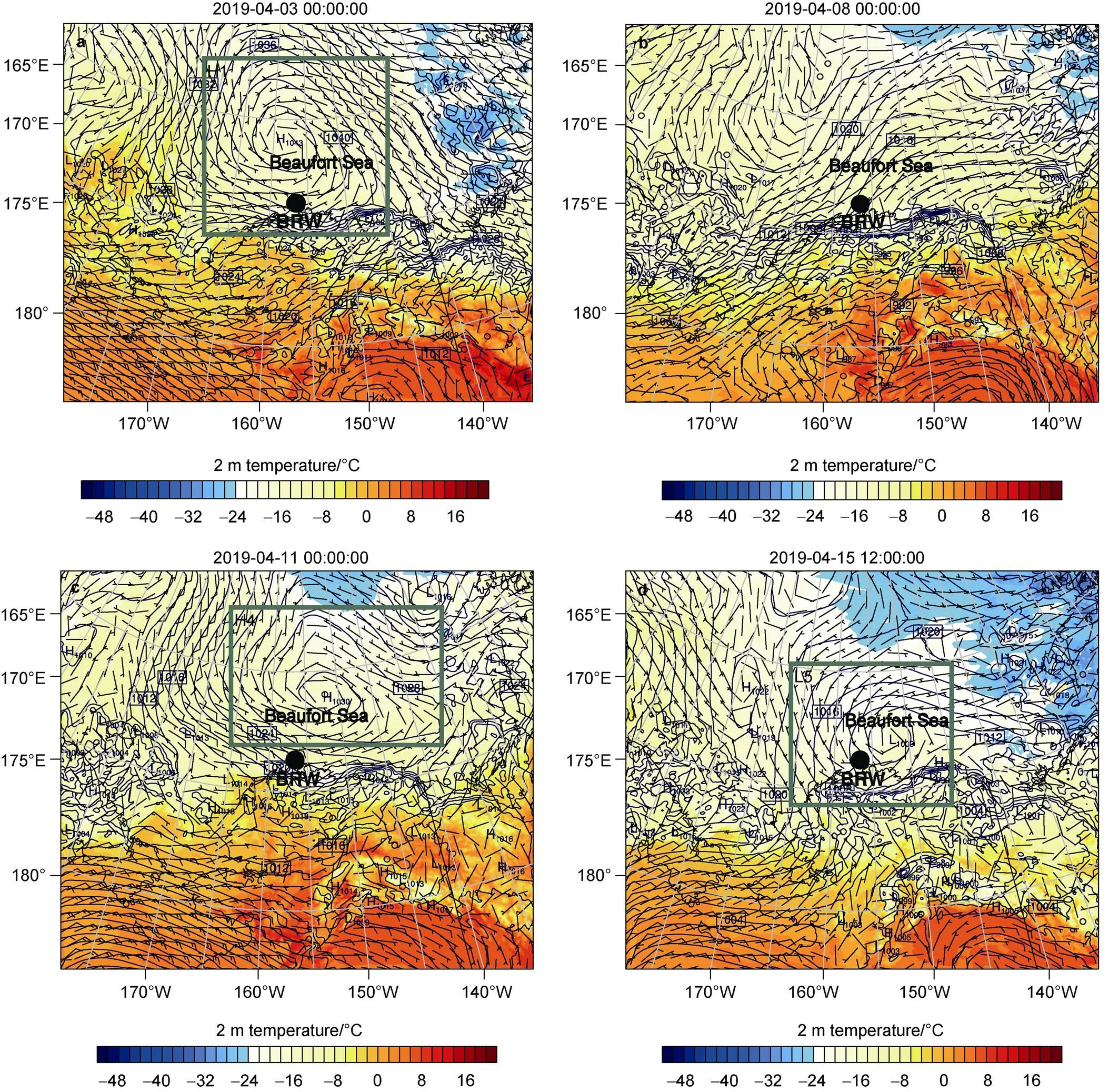
Figure 7 Sea level pressure, 2 m temperature and 10 m wind in simulations of BRW. The times in Figure 7 (a–d) are consistent with those in Figure 6 (a–d). Different weather systems (i.e., cyclones and anticyclones) are marked using rectangles and their names are displayed in the top of the rectangles. The location of the BRW station is also indicated using black points.

We also assessed the WRF model performance in simulating weather systems in the Arctic during the analyzed time period, and we found that the WRF model can successfully capture the variations of these weather systems such as cyclones and anticyclones.

The findings obtained in this study can provide additional evidences for meteorological predictions in the Arctic. They are potentially helpful in simulating extreme events, supplementing meteorological observations, improving understanding of synoptic changes in the Arctic, and providing meteorological results for predictions of air constituents in the Arctic. In the future, we wish to perform WRF simulations for different years, seasons and multiple stations, so that a long-term model performance in predicting meteorological conditions in the Arctic can be assessed.

Figure 8 Sea level pressure, 2 m temperature and 10 m wind in simulations of SUM. The times in Figure 8 (a–d) are consistent with those in Figure 6 (a–d). Different weather systems (i.e., cyclones and anticyclones) are marked using rectangles and their names are displayed in the top of the rectangles. The location of the SUM station is also indicated using black points.

Zhang T: Conceptualization, data curation, formal analysis, investigation, methodology, resources, software, validation, visualization, writing – original draft preparation, writing–review & editing. Cao L: Conceptualization, funding acquisition, methodology, project administration, supervision, writing – review & editing. Li S M: Data curation, methodology, software. Wang J D: Funding acquisition, project administration.

The meteorological observations of BRW are publicly available at https://gml.noaa.gov/aftp/met/brw/. The meteorological observations of SUM can be obtained from https://gml. noaa.gov/aftp/met/sum/. The FNL data can be found at https://rda.ucar. edu/. The surface weather charts can be downloaded from https://www. wpc.ncep.noaa.gov/archives/web_pages/sfc/sfc_archive.php.

This study is funded by the National Key Research and Development Program of China (Grant no. 2022YFC3701204), the 2023 Outstanding Young Backbone Teacher of Jiangsu “Qinglan” Project (Grant no. R2023Q02) and the National Natural Science Foundation of China (Grant no. 41705103). The authors would like to thank the National Supercomputer Center in Tianjin and the High Performance Computing Center at the Nanjing University of Information Science & Technology for providing the high-performance computing system for calculations. We appreciate three anonymous reviewers and Associate Editor Dr. Sheeba N. Chenoli for their constructive comments that have further improved the manuscript.

Alwarda R, Bognar K, Strong K, et al. 2021. Record springtime stratospheric ozone depletion at 80°N in 2020. EGU General Assembly 2021, online, 19–30 Apr 2021, EGU21-8892, doi: 10.5194/ egusphere-egu21-8892.

AMAP. 2021. Arctic climate change update 2021: key trends and impacts. Summary for policy-makers. Tromsø, Norway, Arctic Monitoring and Assessment Programme (AMAP).

Bhatt U S, Walker D A, Walsh J E, et al. 2014. Implications of Arctic sea ice decline for the earth system. Annu Rev Environ Resour, 39: 57-89, doi:10.1146/annurev-environ-122012-094357.

Bromwich D H, Cassano J J, Klein T, et al. 2001. Mesoscale modeling of katabatic winds over Greenland with the Polar MM5. Mon Weather Rev, 129(9): 2290-2309, doi: 10.1175/1520-0493(2001)129<2290: MMOKWO>2.0.CO;2.

Bromwich D H, Hines K M, Bai L S, et al. 2009. Development and testing of polar weather research and forecasting model: 2. Arctic Ocean. J Geophys Res Atmos, 114, doi: 10.1029/2008jd010300.

Bromwich D H, Otieno F O, Hines K M, et al. 2013. Comprehensive evaluation of polar weather research and forecasting model performance in the Antarctic. J Geophys Res Atmos, 118(2): 274-292, doi:10.1029/ 2012jd018139.

Cao L, Li S M, Gu Y C, et al. 2023. A three-dimensional simulation and process analysis of tropospheric ozone depletion events (ODEs) during the springtime in the Arctic using CMAQ (Community Multiscale Air Quality Modeling System). Atmos Chem Phys, 23(5): 3363-3382, doi:10.5194/acp-23-3363-2023.

Carvalho D, Rocha A, Gómez-Gesteira M, et al. 2014. Sensitivity of the WRF model wind simulation and wind energy production estimates to planetary boundary layer parameterizations for onshore and offshore areas in the Iberian Peninsula. Appl Energy, 135: 234-246, doi:10. 1016/j.apenergy.2014.08.082.

Carvalho D, Rocha A, Santos C S, et al. 2013. Wind resource modelling in complex terrain using different mesoscale–microscale coupling techniques. Appl Energy, 108: 493-504, doi:10.1016/j.apenergy.2013. 03.074.

Cassano J J, Box J E, Bromwich D H, et al. 2001. Evaluation of Polar MM5 simulations of Greenland’s atmospheric circulation. J Geophys Res Atmos, 106(D24): 33867-33889, doi: 10.1029/2001JD900044.

Cassano J J, Higgins M E, Seefeldt M W. 2011. Performance of the weather research and forecasting model for month-long pan-Arctic simulations. Mon Weather Rev, 139(11): 3469-3488, doi:10.1175/ mwr-d-10-05065.1.

Dong H T, Cao S Y, Takemi T, et al. 2018. WRF simulation of surface wind in high latitudes. J Wind Eng Ind Aerodyn, 179: 287-296, doi:10.1016/j.jweia.2018.06.009.

Emery C, Liu Z, Russell A G, et al. 2017. Recommendations on statistics and benchmarks to assess photochemical model performance. J Air Waste Manag Assoc, 67(5): 582-598, doi:10.1080/10962247.2016. 1265027.

Friedl M A, McIver D K, Hodges J F, et al. 2002. Global land cover mapping from MODIS: Algorithms and early results. Remote Sens Environ, 83(1/2): 287-302, doi:10.1016/S0034-4257(02)00078-0.

Friedl M A, Sullamenashe D, Tan B, et al. 2010. MODIS Collection 5 global land cover: algorithm refinements and characterization of new datasets. Remote Sens Environ, 114(1): 168-182, doi:10.1016/j.rse. 2009.08.016.

Helmig D, Oltmans S J, Carlson D, et al. 2007. A review of surface ozone in the polar regions. Atmos Environ, 41(24): 5138-5161, doi:10.1016/j. atmosenv.2006.09.053.

Herrmann M, Sihler H, Frieß U, et al. 2021. Time-dependent 3D simulations of tropospheric ozone depletion events in the Arctic spring using the Weather Research and Forecasting model coupled with Chemistry (WRF-Chem). Atmos Chem Phys, 21(10): 7611-7638, doi:10.5194/acp-21-7611-2021.

Hines K M, Bromwich D H. 2008. Development and testing of polar Weather Research and Forecasting (WRF) model. Part I: Greenland ice sheet meteorology. Mon Weather Rev, 136(6): 1971-1989, doi:10. 1175/2007mwr2112.1.

Hines K M, Bromwich D H, Bai L S, et al. 2015. Sea ice enhancements to Polar WRF. Mon Weather Rev, 143(6): 2363-2385, doi:10.1175/mwr- d-14-00344.1.

Holland M M, Bitz C M, Tremblay B, et al. 2006. Future abrupt reductions in the summer Arctic sea ice. Geophys Res Lett, 33(23), 265-288, doi: 10.1029/2006GL028024.

Hughes C P, Veron D E. 2015. Characterization of low-level winds of southern and coastal Delaware. J Appl Meteorol Climatol, 54(1): 77-93, doi:10.1175/jamc-d-14-0011.1.

Iacono M J, Delamere J S, Mlawer E J, et al. 2008. Radiative forcing by long-lived greenhouse gases: calculations with the AER radiative transfer models. J Geophys Res, 113(D13): D13103, doi:10.1029/ 2008jd009944.

Ingold T, Dunbar M, Ostenso N A, et al. 2023. Arctic. Encyclopedia Britannica. (2023-11-12). https://www.britannica.com/place/Arctic.

Janjić Z I. 1994. The step-mountain eta coordinate model: further developments of the convection, viscous sublayer, and turbulence closure schemes. Mon Wea Rev, 122(5): 927-945, doi:10.1175/1520- 0493(1994)122<0927: tsmecm>2.0.co;2.

Kadaverugu R, Matli C, Biniwale R. 2021. Suitability of WRF model for simulating meteorological variables in rural, semi-urban and urban environments of Central India. Meteorol Atmos Phys, 133(4): 1379-1393, doi:10.1007/s00703-021-00816-y.

King J C, Gadian A, Kirchgaessner A, et al. 2015. Validation of the summertime surface energy budget of Larsen C Ice Shelf (Antarctica) as represented in three high-resolution atmospheric models. J Geophys Res Atmos, 120(4): 1335-1347, doi:10.1002/2014jd022604.

Liu X, Cao J, Xin D. 2022. Wind field numerical simulation in forested regions of complex terrain: a mesoscale study using WRF. J Wind Eng Ind Aerodyn, 222: 104915, doi:10.1016/j.jweia.2022.104915.

Lucas-Picher P, Wulff-Nielsen M, Christensen J H, et al. 2012. Very high resolution regional climate model simulations over Greenland: identifying added value. J Geophys Res Atmos, 117(D2): D02108, doi: 10.1029/2011JD016267.

Manney G L, Santee M L, Rex M, et al. 2011. Unprecedented Arctic ozone loss in 2011. Nature, 478(7370): 469-475, doi: 10.1038/nature10556.

Mellor G L, Yamada T. 1982. Development of a turbulence closure model for geophysical fluid problems. Rev Geophys, 20(4): 851-875, doi:10.1029/rg020i004p00851.

NCEP, NWS, NOAA, U.S. Department of Commerce. 2000. NCEP FNL operational model global tropospheric analyses, continuing from July 1999. (2000-04-12) [2023-04-12], doi: 10.5065/D6M043C6.

Niu G Y, Yang Z L, Mitchell K E, et al. 2011. The community Noah land surface model with multiparameterization options (Noah-MP): 1. Model description and evaluation with local-scale measurements. J Geophys Res Atmos, 116(12): D12109, doi: 10.1029/2010JD015139.

Pyrgou A, Santamouris M, Livada I. 2019. Spatiotemporal analysis of diurnal temperature range: effect of urbanization, cloud cover, solar radiation, and precipitation. Climate, 7(7): 89, doi:10.3390/cli7070089.

Showstack R. 2011. NOAA atmospheric baseline observatories provide key data for researchers. EOS Trans, 92(34): 282-283, doi:10.1029/ 2011eo340002.

Skamarock W C, Klemp J B, Dudhia J, et al. 2019. A description of the advanced research WRF Version 4.1 (No. NCAR/TN-556+STR), doi: 10.5065/1dfh-6p97.

Solbakken K, Birkelund Y, Samuelsen E M. 2021. Evaluation of surface wind using WRF in complex terrain: atmospheric input data and grid spacing. Environ Model Softw, 145: 105182, doi:10.1016/j.envsoft. 2021.105182.

Sokolowsky G A, Clothiaux E E, Baggett C F, et al. 2020. Contributions to the surface downwelling longwave irradiance during Arctic winter at Utqiaġvik (Barrow), Alaska. J Clim, 33(11): 4555-4577, doi:10.1175/ jcli-d-18-0876.1.

Surussavadee C. 2017. Evaluation of tropical near-surface wind forecasts using ground observations. 8th International Renewable Energy Congress (IREC). March 21–23, 2017, Amman, Jordan. IEEE, 1-4, doi:10.1109/IREC.2017.7926006.

Thompson G, Field P R, Rasmussen R M, et al. 2008. Explicit forecasts of winter precipitation using an improved bulk microphysics scheme. Part II: implementation of a new snow parameterization. Mon Weather Rev, 136(12): 5095-5115, doi:10.1175/2008mwr2387.1.

Tiedtke M. 1989. A comprehensive mass flux scheme for cumulus parameterization in large-scale models. Mon Weather Rev, 117(8): 1779-1800, doi:10.1175/1520-0493(1989)117<1779:ACMFSF>2.0.CO;2.

Tse K, Li S, Fung J, et al. 2014. A comparative study of typhoon wind profiles derived from field measurements, meso-scale numerical simulations, and wind tunnel physical modeling. J Wind Eng Ind Aerodyn, 131: 46-58, doi:10.1016/j.jweia.2014.05.001.

Wilson A B, Bromwich D H, Hines K M. 2011. Evaluation of Polar WRF forecasts on the Arctic System Reanalysis domain: surface and upper air analysis. J Geophys Res, 116(D11): D11112, doi:10.1029/ 2010jd015013.

Wilson A B, Bromwich D H, Hines K M. 2012. Evaluation of Polar WRF forecasts on the Arctic System Reanalysis Domain: 2. Atmospheric hydrologic cycle. J Geophys Res, 117(D4): D04107, doi:10.1029/ 2011jd016765.

Yang B, Zhang Y C, Qian Y. 2012. Simulation of urban climate with high-resolution WRF model: a case study in Nanjing, China. Asia Pac J Atmos Sci, 48(3): 227-241, doi:10.1007/s13143-012-0023-5.

Zhan C C, Xie M. 2022. Land use and anthropogenic heat modulate ozone by meteorology: a perspective from the Yangtze River Delta region. Atmos Chem Phys, 22(2): 1351-1371, doi: 10.5194/acp-22-1351-2022.

Zhang C X, Wang Y Q, Hamilton K. 2011. Improved representation of boundary layer clouds over the southeast Pacific in ARW-WRF using a modified tiedtke cumulus parameterization scheme. Mon Weather Rev, 139(11): 3489-3513, doi:10.1175/mwr-d-10-05091.1.

Zhang Y, Bocquet M, Mallet V, et al. 2012. Real-time air quality forecasting, part I: History, techniques, and current status. Atmos Environ, 60: 632-655, doi: 10.1016/j.atmosenv.2012.06.031.

Zhang Y, Wang Y, Hou S, et al. 2022. Reliability of Antarctic air temperature changes from Polar WRF: a comparison with observations and MAR outputs. Atmos Res, 266: 105967, doi:10. 1016/j.atmosres.2021.105967.

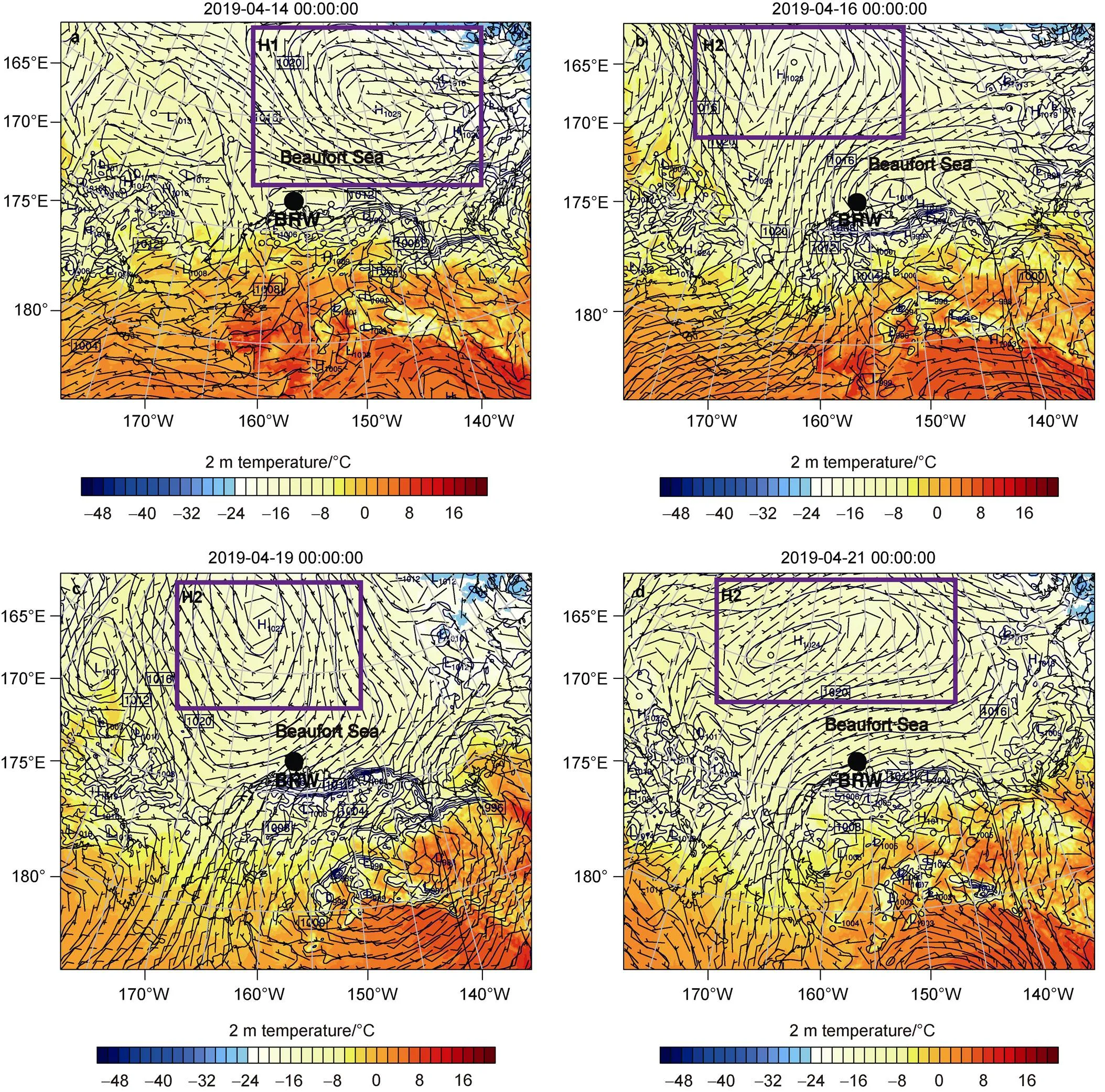
Figure S1 Sea level pressure, 2 m temperature and 10 m wind in simulations of BRW during 00:00 on 14 April to 00:00 on 21 April (UTC, Figures S1a–S1d). Different weather systems (i.e., cyclones and anticyclones) are marked using rectangles and their names are displayed in the top of the rectangles. The location of the BRW station is also indicated using black points.

: Zhang T, Cao L, Li S M, et al. Evaluation of meteorological predictions by the WRF model at Barrow, Alaska and Summit, Greenland in the Arctic in April 2019. Adv Polar Sci, 34(4): 352-367,doi: 10.12429/j.advps.2023.0006

10.12429/j.advps.2023.0006

3 June 2023;

4 November 2023;

30 December 2023

, E-mail: le.cao@nuist.edu.cn