Influence of Arctic Sea-ice Concentration on Extended-range Forecasting of Cold Events in East Asia※

Chunxiang LI, Guokun DAI, Mu MU, Zhe HAN, Xueying MA,Zhina JIANG, Jiayu ZHENG, and Mengbin ZHU

1CAS Key Laboratory of Regional Climate-Environment for Temperate East Asia, Institute of Atmospheric Physics,Chinese Academy of Sciences, Beijing 100029, China

2Department of Atmospheric and Oceanic Sciences and Institute of Atmospheric Sciences,Fudan University, Shanghai 200433, China

3Innovation Center of Ocean and Atmosphere System, Zhuhai Fudan Innovation Research Institute, Zhuhai 518057, China

4CMA-FDU Joint Laboratory of Marine Meteorology, Shanghai 200438, China

5Yantai Vocational College, Yantai 264043, China

6State Key Laboratory of Severe Weather, Chinese Academy of Meteorological Sciences, Beijing 100081, China

7State Key Laboratory of Tropical Oceanography, South China Sea Institute of Oceanology,Chinese Academy of Sciences, Guangzhou 510301, China

8Beijing Institute of Applied Meteorology, Beijing 100029, China

ABSTRACT Utilizing the Community Atmosphere Model, version 4, the influence of Arctic sea-ice concentration (SIC) on the extended-range prediction of three simulated cold events (CEs) in East Asia is investigated.Numerical results show that the Arctic SIC is crucial for the extended-range prediction of CEs in East Asia.The conditional nonlinear optimal perturbation approach is adopted to identify the optimal Arctic SIC perturbations with the largest influence on CE prediction on the extended-range time scale.It shows that the optimal SIC perturbations are more inclined to weaken the CEs and cause large prediction errors in the fourth pentad, as compared with random SIC perturbations under the same constraint.Further diagnosis reveals that the optimal SIC perturbations first modulate the local temperature through the diabatic process, and then influence the remote temperature by horizontal advection and vertical convection terms.Consequently, the optimal SIC perturbations trigger a warming center in East Asia through the propagation of Rossby wave trains, leading to the largest prediction uncertainty of the CEs in the fourth pentad.These results may provide scientific support for targeted observation of Arctic SIC to improve the extended-range CE prediction skill.

Key words: cold event, Arctic sea-ice concentration, extended-range prediction

1.Introduction

Cold events (CEs) are the most conspicuous type of weather event during winter in Eurasia, causing substantial damage to agriculture, transportation, and power infrastructure, as well as considerable disruption to people’s daily lives (Ding and Krishnamurti, 1987; Zhang and Wang,1997; Chen et al., 2004; Gong et al., 2014).In recent decades, several extreme CEs over East Asia have resulted in important impacts on human health.For instance, in late January 2016, much of East Asia experienced a severe cold air process.The cold weather swept through eastern China and also reached Japan, Taiwan, and finally Southeast Asia,producing the first ever snowfall over northern Vietnam and causing the death of 14 people in Thailand and at least 85 in Taiwan (Ma and Zhu, 2019).During January 2018, a recordbreaking blizzard and low temperatures hit northern and central-eastern China, with ice freezing appearing in parts of southern China.This event affected 4.3 million people in 11 provinces, leading to economic losses of more than 0.54 billion US dollars (Wang et al., 2020b).More recently, three striking and impactful extreme cold weather events successively occurred across East Asia and North America during the mid-winter of 2020/21 (Luo et al., 2020; Dai et al.,2022; Zhang et al., 2022).It is, therefore, of great importance to predict such weather events skillfully at a lead time of 2–3 weeks, thereby allowing for early warnings and adequate mitigation strategies (White et al., 2017).

Coinciding with the continued Arctic sea-ice loss, cold winters and CEs have been observed to be more frequent and intense in the past few years over Europe, East Asia, Central Asia, and the eastern United States (Tang et al., 2013;Francis and Vavrus, 2015; Overland et al., 2015; Luo et al.,2016a; Francis et al., 2017; He et al., 2020; Simmonds and Li, 2021).Some studies have suggested that the decreased sea ice in the Arctic has led to a wavier jet stream and slower propagating Rossby waves because of a reduced meridional gradient of the air temperature (Deser et al., 2015;Ronalds et al., 2018; Matsumura and Kosaka, 2019).These changes in the large-scale atmospheric circulation favor blocking over higher latitudes (Liu et al., 2012; Luo et al., 2018,2019a), resulting in more frequent and severe cold-air outbreaks in the midlatitudes over the Northern Hemisphere(Liu et al., 2012; Screen and Simmonds, 2013; Mori et al.,2014; Luo et al., 2017; Vavrus et al., 2017).In particular,sea-ice changes in the Barents–Kara Sea (BKS) have important impacts on the midlatitude cold extremes (Inoue et al.,2012; García-Serrano et al., 2015; Koenigk et al., 2016; Luo et al., 2016a; Yang et al., 2016; Zhang et al., 2018; Li et al.,2021).Such potential weather linkages are mediated by the meridional gradient of background tropospheric potential vorticity (Luo et al., 2019b).

Extended-range predictions of extreme CEs are of great importance owing to their widespread applications in agriculture, urban planning, energy, tourism, and health sectors.Also, continued improvement in extended-range predictions is beneficial to policymakers.Recent studies with operational models at major numerical weather prediction centers demonstrate that skillful forecasts for regular systems may be locally achievable at different spatial and temporal scales(e.g., at extended-range or subseasonal-to-seasonal time scales) (Buizza and Leutbecher, 2015; Selz, 2019; Zhang et al., 2019; Judt, 2020).For example, Vitart et al.(2014)and Buizza and Leutbecher (2015) indicated that the forecast skill horizon for large-scale and low-frequency atmospheric phenomena has been extended to several weeks.Recent studies have found that the deterministic predictability limit of the North Atlantic Oscillation (NAO) is approximately 10–20 days (Scaife et al., 2014; Ferranti et al., 2015;Domeisen et al., 2018).Furthermore, it has recently been shown that the predictability of large-scale and long-lasting Ural blocking (UB) events can reach four pentads (Ma et al.,2022).These findings hint at the potential for CE prediction at extended-range time scales.

From the synoptic perspective, the potential predictors of winter extreme CEs, such as the NAO (Jung et al., 2011;Ferranti et al., 2018) and blocking (Jiang and Wang, 2012),have been investigated as nonlinear initial value problems,which are greatly influenced by initial perturbations (Benedict et al., 2004; Mu and Jiang, 2011; Jiang et al., 2015).Scientists have examined their predictability by using the conditional nonlinear optimal perturbation (CNOP) method (Mu et al.,2003).For instance, Mu and Jiang (2011) compared the similarity of the optimal precursors that trigger blocking onset and the optimally growing initial errors in its predictions.Jiang et al.(2015) investigated the role of nonlinear processes in both the onset and phase-strength asymmetry of the NAO by comparing NAO events triggered by linear optimal perturbation and CNOP.

The predictability sources for weather systems come not only from the atmosphere itself, but also the land, ocean,and sea-ice conditions (Liu et al., 2017).Boundary conditions like the Arctic sea-ice concentration (SIC) are crucial for extreme event predictions in winter (Dai and Mu, 2020; Ma et al., 2022).Arctic sea ice has been observed by satellites since 1979, and the estimates of sea-ice area and thickness rely on a number of geophysical parameters, which introduce unavoidable uncertainties (Giles et al., 2007; Stroeve and Notz, 2018).These inevitable errors in observational data lead to large uncertainties in the specification of boundary conditions (Lorenz, 1969; Zou and Kuo, 1996; Reichler and Roads, 2003).

Observational and numerical results both show that atmospheric circulation may manifest a response to sea surface temperature (SST) and sea-ice fluctuations within a few weeks (Deser et al., 2007; Frankignoul et al., 2014; Luo et al., 2021; Zhuo et al., 2023).Utilizing a numerical model,Semmler et al.(2016) investigated the fast atmospheric response to sudden Arctic sea-ice thinning by introducing a 10-K sea-ice surface temperature warming.Recently,Simon et al.(2020) examined the direct response of the atmospheric circulation to the Arctic sea-ice loss with a relatively short response time (i.e., a few weeks to a couple of months), as opposed to the indirect response that could be due to remote sea ice–driven changes in SST or the land surface state.Motivated by previous studies, there could be a fast response of extreme CEs to the SIC fluctuations on the extended-range scale.However, it is still unclear how Arctic sea ice influences extreme CEs on the extended-range scale.

Moreover, it is unknown what kind of SIC errors are responsible for the biases in CE predictions.Recently,Wang and Mu (2015) extended the CNOP approach to explore the uncertainties in boundary conditions that lead to the largest forecast error.This updated method is denoted as CNOP-B, and it is distinct from the CNOP approach that addresses initial errors (denoted as CNOP-I).Subsequently,Ma et al.(2022) applied the approach to investigate the UB predictability problems concerning the perturbations in the Arctic SIC three pentads in advance of the UB onset; that is,identification of the Arctic SIC perturbation that leads to the greatest growth of prediction error.Inspired by previous studies, we examine the influence of the SIC perturbations under the hypothesis that the prediction skill of CEs may extend beyond the lead time of 3 weeks, the source of which may be partially attributable to boundary conditions such as Arctic sea ice.

In this paper, we adopt the technique introduced in Ma et al.(2022) and extend the analysis to CEs.The goal of this study is to identify the specific SIC perturbations that lead to the largest errors in CEs at the optimization time with a given physical constraint, and assess their influence on the CEs.The region of East Asia (105°E–135°E, 35°N–55°N;red box in Fig.1) is the focus of this study.In summary, we conduct idealized modeling experiments using the Community Atmosphere Model, version 4 (CAM4), to investigate the following questions: (1) What kind of SIC perturbations in the Arctic can lead to the largest forecast errors of CEs in East Asia under given boundary constraint conditions? (2)How do the SIC perturbations remotely affect the prediction of CEs on extended-range time scales? Addressing these issues will provide further understanding of error sources for CE predictions.It can also help us to identify sensitive areas where observations can have the greatest impacts on predictions, thereby improving the prediction of CEs.

Following this introduction, section 2 describes the methods, including the CNOP-B procedure and objective function, as well as the model and reanalysis data used in this study.Section 3 first examines the ability of the model in simulating CEs, and then evaluates the effect of Artic SIC on the simulated CEs.Based on three CEs, the optimal SIC perturbations, which lead to the greatest growth of prediction error for CEs, and the related mechanism, are investigated in section 4.In the final section, we provide a summary,some concluding remarks, and an outlook for future work.

2.Data and methods

2.1.Data

A number of daily meteorological fields during the boreal winter (December–February; DJF) are obtained from ERA-Interim at a 1.0° × 1.0° grid resolution (Dee et al.,2011).We use the atmospheric variables including 2-m surface air temperature (SAT), sea level pressure (SLP), geopotential height at 500 hPa (Z500), and zonal wind at 200 hPa(U200), from 1979/80 to 2017/18 (1980–2018), to assess the meteorological conditions and the synoptic patterns associated with extreme CEs over East Asia.The daily oceanic variables include SST and SIC ranging from January 1982 to December 2001.

2.2.Model experiments

Although the ocean plays a critical role in the response of the atmosphere to sea-ice changes–primarily through its thermal inertia and dynamical effects, an atmosphere-only model is chosen here to explore how Arctic sea ice influences extreme CEs on the extended-range scale, with no interference from ocean processes.The Community Atmosphere Model, version 4 (CAM4), with prescribed SST and SIC conditions, is used in this study.It uses a finite volume dynamic core with a hybrid sigma-pressure vertical coordinate.The horizontal resolution for CAM4 is 0.9° latitude by 1.25° longitude (～100 km), with 26 vertical levels up to 3.5 hPa (Neale et al., 2013).Consistent with the default forcing, the calendar means of daily SST and SIC during January 1982 to December 2001 from ERA-Interim, with a 1.0° × 1.0° spatial grid resolution, are adopted as the model boundary conditions.A 51-year control (CTRL) simulation is conducted using a repeating cycle of SST and SIC derived from the 1982–2001 climatology in ERA-Interim.The first year of model data is discarded as the model spin-up period, and the remaining 50 years of model data are used for analysis,which is referred to as the CTRL experiment.Dai et al.(2021) demonstrated that CAM4 can successfully describe the atmospheric circulation during wintertime by comparison with reanalysis data.

2.3.Definition of a CE

A one-dimensional East Asian temperature index(EATI) is used to identify extreme CEs.The index is defined in terms of the domain-averaged SAT anomaly over East Asia (35°–55°N, 105°–135°E).Specifically, the daily anomaly is calculated as the deviation from the long-term climatology for each calendar day.Then, we rank the EATI values to calculate the 10th percentile on the calendar day using a 5-day moving window centered on the day of interest, following the method described in Zwiers and Zhang(2009).An extreme CE is identified when the EATI falls below the calendar day 10th percentile and persists for more than 5 days.Day 0 for a CE is defined as the onset day when the EATI first reaches its criterion.

2.4.CNOP-B and objective function

The CNOP-B method is used to investigate the influence of Artic SIC on CEs.CNOP-B denotes the specific boundary perturbation that results in the largest nonlinear evolution of atmospheric anomalies at the optimization time under a given physical constraint (Wang and Mu, 2015; Wang et al.,2020a).The definitions of the constraint optimization problem are the same as in Dai et al.(2023).

We superimpose the boundary perturbation three pentads before the CE onset day and integrate the model for 20 days.The reason for adding the SIC perturbation 15 days in advance is explained in section 3.3.Since our focus is on the extended-range scale, the forecasts are generated for 5-day means, such as pentad 1 (P1; day -15 to day -11), pentad 2 (P2; day -10 to day -6), pentad 3 (P3; day -5 to day -1),and pentad 4 (P4; day 0 to day 4).Considering that the persistence of CEs is approximately 5 days, the fourth pentad corresponds to the CE duration.Therefore, the fourth pentad average EATI [domain-averaged SAT anomaly over (35°–55°N,105°–135°E)] difference caused by the boundary perturbation b0at the optimization time is defined as the objective function,Jb0,δ:Here, B0is the boundary condition in reference state and b0is the Arctic SIC perturbation.In particular, B0is the calendar means of SIC ranging from 1982 to 2001.Meanwhile, b0denotes Arctic SIC perturbations covering from 40°N to 90°N (including the Okhotsk Sea) and is time-independent,which indicates the SIC perturbations are unchanged during the integration period.are the P4 average EATI values derived from the model integration without and with boundary perturbation b0, respectively.Therefore,the CNOP-B is the boundary perturbation that causes the largest EATI difference in P4.It should be noted that, in this study, the “anomaly” is calculated by subtracting the climatology from the CTRL run, and “response” refers to the difference from the reference state.

The description of constraint of the Arctic SIC perturbations parallels that of Ma et al.(2022).Moreover, a particle swarm optimization (PSO) intelligent algorithm (Kennedy and Eberhart, 1995; Shi and Eberhart, 1999; Song et al.,2023) is used to solve nonlinear optimization, following Yang et al.(2020).However, due to the high dimension in Arctic SIC perturbations, dimension reduction should be conducted.Similar to that in Ma et al.(2022), we adopt the rotated empirical orthogonal function (EOF) to reduce the dimensions of Arctic SIC perturbations.Compared to unrotated EOFs, rotated EOFs can provide a more accurate and physically interpretable representation of the underlying climate variability (Huth and Beranová, 2021).Here, the first 20 eigenvectors are chosen since they can explain more than 80% of the daily Arctic SIC variability in winter.Considering the efficient optimization as well as computational resources, we apply 20 particles with 20 iteration steps to solve the nonlinear optimization problem.

3.The simulated extreme CEs

3.1.CE simulation ability

According to the definition of a CE, there are 18 CEs over eastern Asia during the winters of 1979–2018.Meanwhile, 20 cases are identified in the 50-year CTRL simulation.The synoptic configuration of the CEs in terms of the composite anomalies of SLP, Z500, and U200 during the CE life cycle is shown in Fig.1.Here, we focus on the North Atlantic–Northwest Pacific region (25°–90°N, 30°W–160°E), where the NAO, UB, and East Asian trough–the dominant circulation structures associated with CEs–are most evident.For SLP, both observation and simulation show a continental-scale anticyclonic anomaly north of 40°N, indicating a strengthened UB (Figs.1a and b).In the middle troposphere, there is a Z500 anomaly over the Eurasian continent, with an anticyclonic anomaly near the Ural Mountains and a cyclonic anomaly over East Asia and the surrounding oceans (Figs.1c and d).In the upper troposphere, the East Asian jet stream near 30°N–45°N accelerates, and a westerly flow to the north weakens (Figs.1e and f).In general, large-scale atmospheric circulations, such as the UB and the strengthened East Asian jet stream, favor the cold waves over East Asia.Qualitatively, CAM4 reproduces the typical anomalous atmospheric circulations for the CEs well, with spatial correlation coefficients larger than 0.80,indicating that the model has the ability to simulate the atmospheric circulations of CEs as observed.

3.2.The CE cases

Two recent CE cases occurred under similar atmospheric circulation backgrounds: one during 18–23 January 2016,and the other during 22–28 January 2018.That is, both extreme events were triggered by an intensified UB high, as well as intensification and southward extension of the Siberian high.Studying such recent cases may help us to better predict upcoming extreme CEs in the future.Taking these two observational events as references, there are three cases (denoted case 1, case 2, and case 3) with similar circulations to them in the CTRL simulation.We have examined the predictability of the selected three CEs and found that they have predictability of 4 pentads (not shown).Therefore,these cases are used to explore the Arctic SIC influence on their evolutions.

For the three selected cases in CTRL, Fig.2 shows the 2-day mean evolution of Z500 anomalies and wind anomalies at 850 hPa from day -4 to day +2 along with the Z500 climatology from the CTRL simulation.The basic common properties of the circulation patterns associated with the three CE cases show an anticyclonic anomaly over North Eurasia and cyclonic anomalies over East Asia and the North Atlantic.With the development of the CEs, the anticyclone undergoes a process of developing and strengthening northward before the outbreak of each CE, and then one of retreating and weakening southward (not shown).The dominance of the anticyclone over the extratropics promotes the advection of polar air masses along its downstream cyclonic component and triggers a cold-air outbreak in East Asia.However, several regional differences exist among the cases.For example,case 2 shows a more progressive ridge–trough pattern,while there is a shift of the anticyclone northeastward in case 3 compared with case 1.Moreover, case 3 may be caused by a weak stratospheric polar vortex and a negative Arctic Oscillation (AO) pattern.Nevertheless, all three cases develop into CE events in pentad 4.

3.3.Responses of CEs to SIC perturbations

In order to determine the response time of CEs to SIC perturbations, some sensitivity experiments are conducted.There are 40 Arctic SIC perturbations obtained as 40 winter anomalies for the period 1979–2018.These SIC perturbations have been superimposed on the boundary conditions 15 days, 10 days, and 5 days in advance of the CE onset, respectively.We then integrate the numerical model with these SIC perturbations for 30 days.

The numerical results of the CE responses to Arctic SIC perturbations with different start times are depicted in Fig.3.An earlier study showed an obvious response of the NAO to sudden sea-ice thinning over 10 days (Dai et al.,2021).Similarly, here, when the Arctic SIC perturbation begins 15 days ahead of the CE onset, there is a significant impact of Arctic SIC on the CE prediction, with an obvious response of EATI after 11 days (day -4; Figs.3a, d and g).With a start time of 10 days ahead of CE onset, Arctic SIC perturbations show almost no influence on the prediction of CE onset (day 0), but cause some uncertainties during the CE decay period (Figs.3b, e and h).Nevertheless, the SIC perturbations at 5 days in advance have little influence on the CE onset or development forecast, but contribute to some uncertainties 10 days after the CE onset (Figs.3c, f and i).

Sensitivity experiments show that the CE event has an obvious response to Arctic SIC perturbation after 10 days,regardless of the time when the perturbation starts.Moreover, if the SIC perturbations start at day -15, they could influence the entire CE life cycle, including its onset and decay stages.Therefore, the optimization calculation is conducted with a start time of 15 days in advance of the CE onset.

4.CNOP-B results

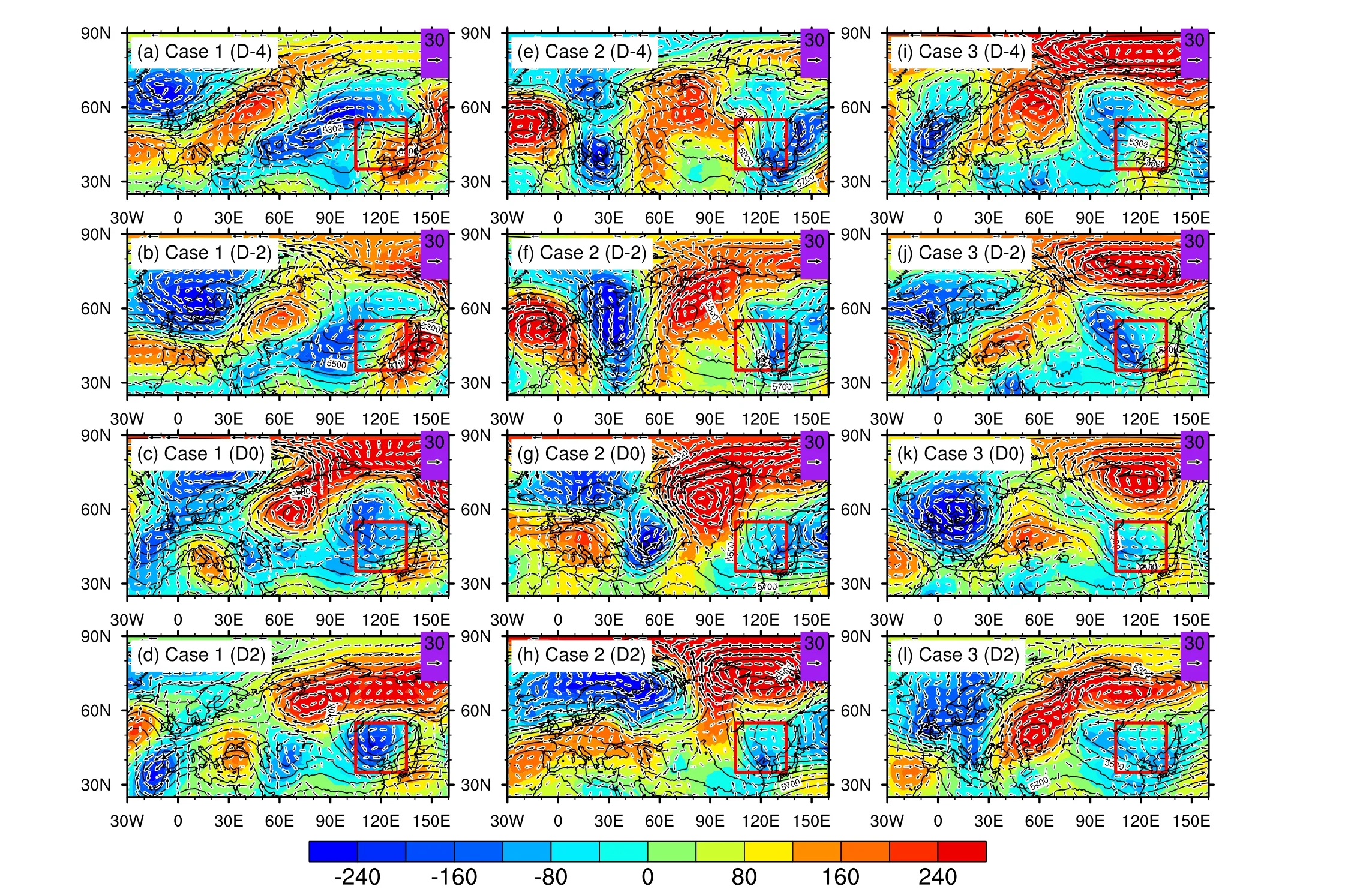
Fig.2.(a–d) Evolutions of the Z500 (contours; units: gpm) and its anomaly (shaded; units: gpm) and wind anomaly at 850 hPa (vectors; units: m s-1) for case 1 at day -4, -2, 0, and 2 with respect to the climatology.Panels (e–h) and (i–l) are similar to (a–d) but for case 2 and case 3, respectively.The contour interval for Z500 is 100 gpm.The red box indicates East Asia (35°–55°N, 105°–135°E).

To identify the specific type of boundary perturbations that lead to the largest nonlinear evolution of CEs, iteration has been carried out by solving the aforementioned nonlinear optimization problem.A simulation with the CAM4 model without sea-ice perturbation serves as the reference integration.

4.1.CNOP-Bs for three cases

Taking the CTRL forecast as the reference state, the optimal Arctic SIC perturbation can be obtained by solving Eq.(1) for the corresponding nonlinear optimization problem.Figure 4 shows the spatial structure of the CNOP-Bs for three cases.It can be seen that the CNOP-B for case 1 shows negative SIC perturbations in the Greenland Sea(GS), BKS, Sea of Okhotsk (OKS), and Bering and Chukchi seas (Fig.4a).Meanwhile, the CNOP-B for case 2 shows sea-ice loss in the vicinity of the GS and BKS but an increase in the OKS and Bering Sea (Fig.4b).Moreover,the CNOP-B for case 3 is characterized by positive SIC perturbations in Baffin Bay, the GS, and BKS, accompanied by negative perturbations over the Bering Sea (Fig.4c).The results suggest that the CNOP-Bs seem to be case-dependent.To examine whether the calculation of the CNOP-Btype perturbations are reliable, additional experiments are conducted for the three cases.Similar to the procedure of Ma et al.(2022), we have added 50 different random SIC perturbations with very small amplitudes to the CNOP-Bs in each case, satisfying the physical constraint in Eq.(3) of Ma et al.(2022).Integration results (not shown) denote that even a slight shift from the CNOP-Bs could lead to a decrease in the objective function value.These confirm that the obtained CNOP-B type SIC perturbations cause the largest uncertainty in East Asia CE predictions in the fourth pentad, as compared with random SIC perturbations under the same constraint.

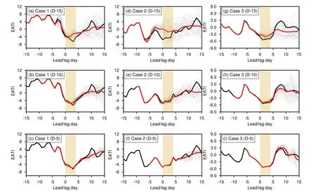
Fig.3.EAT index (EATI; units: K) responses to the Arctic SIC anomaly with different start times.Panels (a–c) correspond to the Arctic SIC anomaly 15, 10, and 5 days in advance of the case 1 onset, respectively.Panels (d–f) and (g–i) are similar to (a–c) but for the onset of case 2 and case 3, respectively.The black solid lines denote the reference states, dashed black lines correspond to the results derived from 40 SIC perturbations, and solid red lines represent the mean of the 40 dashed black lines.Day 0 represents the onset date and the light-yellow bars highlight the CE period.

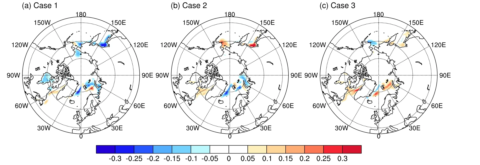
Fig.4.Optimal SIC perturbation for (a) case 1, (b) case 2, and (c) case 3.

Fig.5.Temporal evolutions of the EATI (units: K) triggered by optimal SIC perturbations (red solid lines), 50 random SIC perturbations (dashed black lines), and their reference states (black solid lines) for three cases from day-15 to day 4 relative to the onset of CEs.Day 0 represents the onset date and light-gray bars highlight the CE period.

Next, we superimpose the optimal SIC perturbation on the reference boundary fields in each case and integrate CAM4 over 20 days to explore their effect on the evolution of the CE.The daily variation characteristics of the EATI amplitude flows from fifteen days prior (day -15) to four days after (day +4) the establishment of the CE are investigated.In Fig.5, the black and red solid lines denote the EATI derived from the integration without and with optimal SIC perturbations, respectively.The results show that the EATI curves correspond to the reference state and that the CNOP-Bs behave similarly in the first 11 days, indicating an obvious response of CE events to Arctic sea ice in 11 days (day -4).Eventually, the CNOP-B develops into a warm event in the fourth pentad.We also compare the influence of the random SIC perturbations on CE prediction in sensitivity experiments.We employ 50 sets of random SIC perturbations without any specific spatial structure but having the same constraint and similar amplitude as the CNOP-Bs for each case.The results show that the growth of almost all random perturbations is relatively weak, and their ensemble mean captures well the CEs in the fourth pentad (Fig.5).That is, much smaller objective function values are found in the integrations with these sets of random SIC perturbations than those derived from CNOP-Bs.These indicate that SIC perturbations in specific structures have a marked influence on CE prediction, while random SIC perturbations have little influence.

4.2.Mechanisms of CNOP-B effects on CEs

The previous section identifies the errors with CNOP-B structures over the Arctic sea ice leading to the largest forecast errors in EATI.In this section, the physical processes contributing to the CNOP-B effects on CEs are investigated by decomposing the heat budget balance and examining the corresponding large-scale atmospheric conditions that affect the CEs.Here, the heat budget equation in pressure coordinates (e.g., Hoskins et al., 1989; Nigam, 1994) is decomposed into three terms, denoted as terms A–C respectively.Term A is the horizontal temperature advection, term B represents the vertical adiabatic convection of temperature, and term C denotes diabatic heating/cooling.A detailed description of the equation can be found in Ma et al.(2022); for the sake of conciseness, we only give the main result here.

4.2.1.Case 1

To infer the influence of CNOP-B, we investigate the temporal evolution of the circulation response over the polar cap region (north of 65°N).Figure 6 presents the difference between the two evolutions of the polar cap geopotential height (PCH), zonal-mean zonal wind, and polar cap temperature around the onset dates in case 1.The latitude–time cross sections of the vertical component of Eliassen–Palm(EP) flux vector at 100 hPa and divergence of EP flux at 50 hPa are further given.They, as a proxy for the northern annular mode (Baldwin and Dunkerton, 2001; Baldwin and Thompson, 2009), can be used to estimate the strength and the downward propagation of the stratospheric polar vortex.

It is clear that there are significantly negative stratospheric and upper-tropospheric height anomalies over the entire polar cap during the whole period (from day -15 to day 4) in the reference state.This is a consequence of the anomalously persistent strong polar vortex in case 1.Compared to the reference state, the CNOP-B increases the vertical wave propagation into the stratosphere and leads to a divergence of EP flux over the area north of 50°N from day -6 to day 4 at 100 hPa (Fig.6e).This strengthens the stratospheric polar vortex to a certain extent (Fig.6b) and causes a westerly acceleration (Fig.6c) and decreased temperature (Fig.6d) in the lower troposphere around the polar region from day -4.Consequently, decreased gradients of temperature and pressure are formed between high and middle latitudes, disfavoring the southward propagation of cold air from the Arctic region into the Eurasian continent.

The polar cap response highlights the stratospheric influence over the polar region.Moreover, the contributions of heat budget terms to temperature changes in the lower troposphere (TPL, 750–950 hPa) and the associated physical processes are also examined.The pentad-averaged TPL heat budget analysis results are shown in Figs.7a–d.Similar to Ma et al.(2022), if the local change of temperature in one grid cell is mainly dominated by horizontal temperature advection, vertical adiabatic convection of temperature, and diabatic heating (component A, B and C), the grid cell is shaded green, yellow and red, respectively.We also calculate the proportion of the grid cell (RG) that is dominated by each component relative to the entire region (40°N–90°N)using area weights.The resulting ratios are presented in parentheses in Figs.7a–d.Figures 7e–h, 7i–l, and 7m–p show the temporal evolution of the pentad differences of temperature in the TPL, Z500, and U200 between the CNOP-B and reference state for case 1, respectively.

The spatial distribution of term C shows spread to a larger region compared to other terms in pentad 1 (RG =43.0%; Fig.7a).This suggests that the temperature perturbations in the TPL are mainly affected by the diabatic heating process (term C), which shows a consistent pattern with optimal SIC perturbation in pentad 1.The temperature perturbations in the TPL are mainly positive and located over the BKS where the SIC perturbations are negative.Meanwhile,the response of the atmospheric circulations (Z500 and U200) to the CNOP-B are anomalously weak and also mainly located near the BKS (Figs.7f and m).

Pentad 2 exhibits a “negative–positive–negative” wavelike pattern of Z500 and temperature response in the Kara Sea, North Siberian Lowland, and northeast of the western North Pacific (WNP).In pentad 3, there are two dipole-like atmospheric circulation patterns with an intensification of Z500 over northern Europe/the Okhotsk Sea and a decrease over southern Europe/the subtropical WNP region.The height responses are reminiscent of the positive phase of teleconnection patterns (eastward-shifted NAO) and the western Pacific (Wallace and Gutzler, 1981), which drive the temperature to increase over East Asia in the following pentad (Park and Ahn, 2016).

The coolings in the TPL over the polar cap region are mainly dominated by the thermal advection and convection processes (terms A and B) in the fourth pentad (Fig.6d).Correspondingly, CNOP-B decreases the East Asian subtropical jet stream but increases the East Asian polar front jet stream in the upper troposphere compared to the reference state(Fig.7p).The Z500 composite (Fig.7k) reveals a zonal wave-like pattern triggered from the polar regions associated with the CNOP-B pattern of SIC perturbations (Yao et al.,2017; Ye and Messori, 2020).That is, UB has been suppressed, associated with a decreased wind gradient (northeasterly) over East Asia at 850 hPa (not shown).Therefore,CNOP-B warms the SAT significantly in East Asia in the fourth pentad.

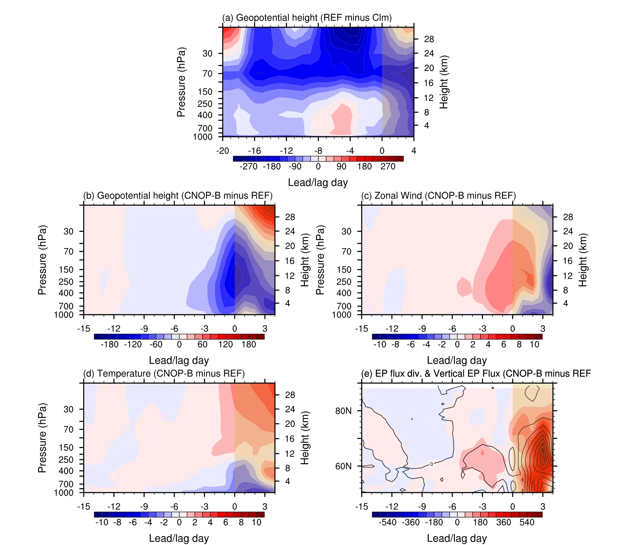
Fig.6.Time–altitude evolution of the polar cap (65°–90°N, 0°–360°E) mean (a) geopotential height anomaly (units:gpm) in the reference state (REF), (b) geopotential height (units: gpm), (c) zonal wind (units: m s-1), and(d) temperature (units: K) response to the CNOP-B.(e) Time–latitude response of the EP-flux divergence anomaly at 50 hPa (shading; units: m s-1) and the vertical component of EP flux at 100 hPa (contours; interval: 10 hPa m s-2;negative contours are dashed) for case 1.The x-axis is time, with lag 0 indicating the CE onset day.Note that the preceding days from REF [panel (a)] have been extended to 20 days leading up to the hindcast start in order to show the evolution of the geopotential height of REF.

4.2.2.Case 2

In the reference state of case 2, there are positive stratospheric and upper-tropospheric PCH anomalies before day-4, suggesting a weakened polar vortex about a pentad in advance (Fig.8a).However, simulation using CNOP-B shows that the downward EP flux at 100 hPa is found over the latitudes of 45°–60°N during day -6 to day 0, and this reduced EP flux is linked to the EP flux divergence at 50 hPa at high latitudes (Fig.8e).The reduced convergence of planetary wave EP flux at high latitudes leads to lower wave-induced drag on the mean flow, which is related to the acceleration of westerly winds (Fig.8c), an increased stratospheric weak vortex (Fig.8b), and a decreased temperature in the troposphere (Fig.8d).These responses provide a detrimental background for the development of CE events in East Asia.

In pentad 1, the temperature perturbations in the TPL are mainly influenced by the diabatic heating process (term C, RG = 38.8%) (Fig.9a).Meanwhile, the response to seaice perturbation in the atmospheric circulation is concentrated in the troposphere.This is particularly localized in the increase (decrease) of the TPL and decrease (increase) of the Z500 over the GS (Chukchi Sea) associated with the declined (enhanced) SIC (Figs.9e and i).In the following three pentads, the horizontal advection term becomes the dominant heat term (Figs.10b–d; RG = 47.2%–47.5%).Correspondingly, it shows a cyclonic anomaly over the Laptev Sea and Kara Sea but anticyclonic anomaly appearing elsewhere in the Arctic at the middle level in the second pentad(Z500, Fig.9j).In the third pentad, enhanced westerly winds at 500 hPa are found in the UB sector (not shown),tend to change the Z500 field, and weaken blocking circulations (Luo et al., 2017; Yao et al., 2017; Ma et al., 2022;Zhuo et al., 2022).This produces two north–south dipoles,with negative Z500 in Baffin Bay–Hudson Bay and the Ural Mountains, and positive Z500 over the North Atlantic and Europe (Fig.9k).Subsequently, the latter dipole shifts eastward, with the positive center covering East Asia in the fourth pentad (Fig.9l).Meanwhile, the Siberian high weakens(not shown), and the East Asian trough shallows (Fig.9l).The East Asian jet stream in the upper troposphere weakens as well (Fig.9p), and the regional temperature in East Asia increases as a consequence (Fig.9h).

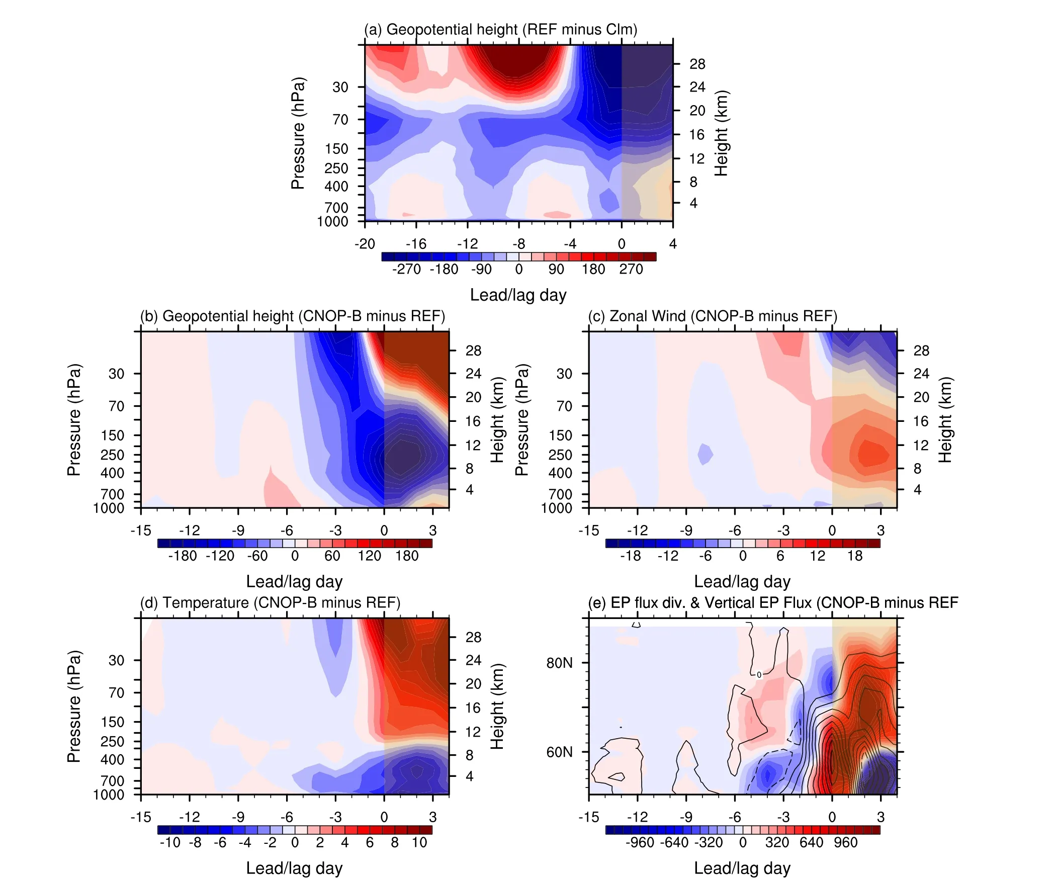
Fig.8.As in Fig.6 but for case 2.The contour interval in (e) is 20 hPa m s-2.

4.2.3.Case 3

In case 3, positive PCH anomalies are present from the surface to mid-stratosphere throughout the four pentads in the reference state.This indicates a suppression of the stratospheric vortex and a negative phase of the AO at the surface,consistent with the above-normal Z500 throughout the Arctic(Figs.2i–l).Plots of the EP flux and its divergence (Fig.10e)show that a north–south dipole of EP flux divergence evolves in the mid–high latitudes during day -4 to day 0.This indicates that the planetary waves tend to propagate equatorward and are associated with EP-flux divergence in the north and convergence in the south, representing the westerly and easterly zonal momentum force exerted by planetary waves on the mean flow, respectively.Correspondingly,there is an enhanced westerly zonal wind in the polar cap region (Fig.10c and Fig.11o), which is unfavorable for cold air masses invading East Asia.In contrast, the polar cap–averaged geopotential height (Fig.10c) and temperature(Fig.10e) show increases throughout the whole level, suggesting increased gradients of temperature and pressure between high and middle latitudes.

The local temperature changes are contributed by the diabatic term (term C) in the first pentad, but by the horizontal advection (term A) in the last three pentads, compared with the other two terms, as shown in Figs.11a–d.Cooling in the TPL over Baffin Bay is observed in the first two pentads, corresponding to positive sea-ice perturbation.(Figs.11e and f).Prior to the sudden warming in East Asia, the difference in U200 shows that a negative-over-positive dipole anomaly is located over a region stretching from the BKS to the south side of the Ural Mountains, ranging from 30° to 90°E, since the third pentad (Fig.11o).Such an intensified westerly wind in the upstream region is unfavorable for the southward transportation of cold air to East Asia.Figure 11k further shows that positive and negative Z500 anomalies are found in the region of the BKS and central Siberia, respectively.These dipole anomalies are strengthened and shifted westward and southward during the fourth pentad.Specifically,the differences of Z500 feature relatively strong cyclonic circulation in northeastern Asia and anticyclonic circulation in East Asia (Fig.11l).Under these circulation conditions, northeasterly winds in the lower troposphere over East Asia decelerate because of the weakened meridional gradient of geopotential height.Consequently, temperature is higher than normal over East Asia (Fig.11h).

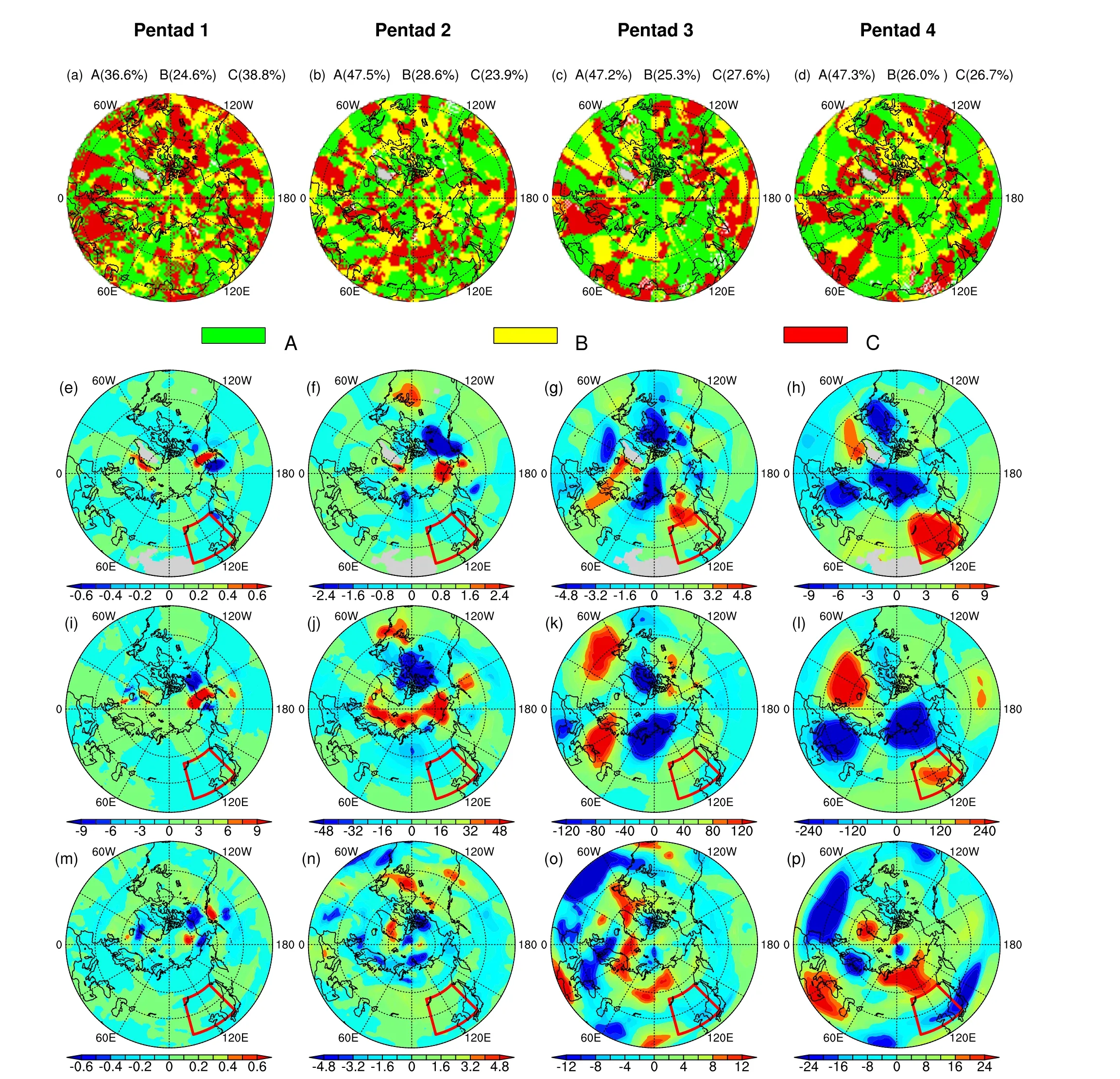
Fig.9.As in Fig.7 but for case 2.

5.Discussion and conclusion

There is an increasing requirement for accurate and reliable extended-range forecasts, especially for extreme weather events because of their profound impacts.In this paper, we investigate the influence of Arctic SIC uncertainty on the extended-range prediction of extreme CEs in East Asia.Based on the rotated EOF-based PSO algorithm, the CNOP-B approach is applied to the identification of the optimal Arctic SIC perturbations that lead to the largest prediction error in CEs over East Asia in the fourth pentad.The results suggest that the CNOP-B perturbations in Arctic Asia can cause the largest error growth compared with other SIC perturbations at extended-range scale for extreme CEs in East Asia.The CNOP-B is therefore the most sensitive SIC perturbation and it would have potential for providing the sensitive area for future targeting observations in the Arctic region.The uncertainty of SIC in the Arctic with a specific structure(e.g., CNOP-B) may lead to greater influence on CE predictions than the uncertainty without a spatial structure (i.e., random perturbation).These findings suggest that it is possible to improve the reliability of extended-scale forecasts of CEs by increasing the ensemble spread in the ensemble prediction, and through the assimilation of additional data collected in targeted observation zones.

Heat budget balance analysis is further applied to explore the role of different heat terms in affecting TPL temperature.We find that the major term related to the evolution of temperature is the diabatic heating process and horizontal advection in the first and fourth pentads respectively, which is similar to the result reported in Ma et al.(2022).On the other hand, we find that both the vertical adiabatic convection and the horizontal advection play an important role for temperature change in the second and third pentads.

Correspondingly, the CNOP-Bs in case 1 and case 2 lead to a divergence of EP flux over the polar cap, decrease the geopotential thickness, and cause a westerly acceleration and temperature decrease in the lower troposphere around the polar region in the third pentad.Consequently, the CNOP-Bs in the Arctic SIC trigger a warming in East Asia through Rossby wave propagation, leading to the largest prediction error of the CEs in the fourth pentad.However, it should be noted that the facilitation of teleconnection from the Arctic basin to the midlatitudes is contingent upon the characteristics of the circulation between these two regions(Rudeva and Simmonds, 2021).For case 3, CNOP-B reduces the negative-over-positive dipole anomaly of U200 over a region stretching from the BKS to the south side of the Ural Mountains and from 30° to 90°E since the third pentad.Such an intensified westerly wind in the upstream region is not conducive to the southward transportation of cold air to East Asia.

It is worth mentioning that the results of modeling studies regarding the impact of Arctic SIC boundary conditions on CE prediction skill at the extended-range scale depend on the model employed in the study.Nonetheless, we can conclude that the present study provides support for a causal link between Arctic SIC uncertainty and CE prediction in East Asia on an extended-range time scale.Moreover, the CNOP-B structures and physical mechanisms for their modulations seem to be case-dependent, which encourages statistical evaluation of the forecast skill with more CE cases.Recently, Han et al.(2023) examined the effect of atmospheric uncertainties in the Arctic on the predictability of CEs in East Asia.It was demonstrated that the CNOP-type initial uncertainty in the Arctic can lead to a CE appearing as a normal or warm event at the extended-scale range.Moreover, they found that the spatial patterns of the CNOP-type initial uncertainty in the three cases also seem to be casedependent, due to the different initial conditions.Evidence collected in their contexts is similar to ours, and consistent findings across a variety of contexts will support our results.However, further work with investigation into the possible reasons needs to be carried out in the future.

Due to the significant case-dependent characteristic of CNOP-type perturbations and its resultant largest prediction errors, it is reasonable to consider the CNOP method as a candidate in SIC adaptive observation to improve the forecast skill for CEs.However, we have investigated the influence of SIC perturbations in the Arctic on CE prediction only based on a control forecast using idealized experiments,rather than an ensemble of forecasts.This inspires further exploration of CE prediction through ensemble approaches,to capture the effects of case-dependent SIC uncertainties and their evolution in the forecast.In addition to the Arctic SIC, CE activity in East Asia is also affected by Arctic seaice thickness and SST (Luo et al., 2016b; Yao et al., 2017).For instance, the sea surface temperature anomaly in the pattern of the North Atlantic tripole exerts its influence on CEs via the NAO and UB circulation (Chen et al., 2021).However, the role of the Arctic SST in CE formation has not been discussed in this study.Moreover, it should be noted that the SST usually warms along with the melting and thinning of sea ice.The combined effects of the SIC and SST may result in larger influences on CEs (Zhang et al., 2022).Furthermore, both the initial and boundary conditions are crucial for extended-range prediction (Baldwin et al., 2003;Vitart, 2004; Vitart and Robertson, 2018).In this study, we mainly discuss the influence of Arctic SIC uncertainty on CE evolution.The role of initial uncertainties in the atmosphere will be investigated in a separate paper.

This study only addresses the direct impacts of Arctic sea-ice change on atmospheric circulation and CEs, and neglects the potential role of oceanic feedbacks.In fact, incorporating more comprehensive representations of these boundary forcings, as well as their associated large-scale teleconnections in coupled atmosphere–ocean models, has been found to be important in simulating the response to sea ice (Deser et al., 2016;).However, CAM4 is an atmospheric general circulation model, and the effects of the atmosphere on SIC perturbations are not considered in the present study.Future work by our group will involve investigating the mechanisms of interaction between the SIC and atmosphere in a fully-coupled forecast system.

Acknowledgements.This research was supported by the National Natural Science Foundation of China (Grant Nos.42288101, 41790475, 42175051, and 42005046), the State Key Laboratory of Tropical Oceanography (South China Sea Institute of Oceanology, Chinese Academy of Sciences; Grant No.LTO2109),and the Guangdong Basic and Applied Basic Research Foundation(Grant No.2021A1515011868).We are grateful to TianHe-2(National Supercomputer Center in Guangzhou) for granting us computational resources for carrying out the simulations.The calculations in this work were performed on TianHe-2 and the Atmospheric–Oceanic Numerical Simulation Platform.The authors appreciate the support of the National Supercomputer Center in Guangzhou(NSCC-GZ) and the High Performance Computing Center in the Department of Atmospheric and Oceanic Sciences, Fudan University.The authors thank the European Centre for Medium-range Weather Forecasts for supplying the ERA-Interim data used in this study (https://apps.ecmwf.int/datasets/).