An Improved Prediction Method for Structural Response Analysis of Offshore Wind Turbines

-

(a.State Key Laboratory of Ocean Engineering;b.School of Naval Architecture,Ocean and Civil Engineering,Shanghai Jiao Tong University,Shanghai 200240,China)

Abstract:In order to overcome the shortcomings of the traditional Rosenblatt-IFORM (Inverse-First-Order Reliability Method) environmental contour method, the use of the PCA (Principal Component Analysis)-IFORM contour method is proposed for generating more accurate environmental contours.The environmental contours at a chosen offshore site obtained by using the PCA-IFORM contour method are compared with those obtained by using the Rosenblatt-IFORM environmental contour method,and the accuracy and effectiveness of the PCA-IFORM contour method are convincingly validated.The 50-year extreme structural dynamic responses of a monopile-supported 5 MW offshore wind turbine installed at this chosen offshore site are calculated based on the highest nonlinear sea state from the PCA-IFORM contour method (or the traditional Rosenblatt-IFORM environmental contour method).The calculation results are systematically analyzed and compared,and the necessity and importance of using more realistic environmental contours (such as those generated using the PCA-IFORM contour method)are finally highlighted.

Key words:novel environmental contour method;principal component analysis;inverse-first-order reliability method;extreme structural dynamic response;offshore wind turbine

0 Introduction

In the ship classification rules for designing and building offshore wind turbines,the characteristic responses(extreme responses)are defined regarding a specific return period(e.g.a 50-year design service life).Accurate prediction of these characteristic response values requires correct identification of the long-term extreme sea states.In recent years, the environmental contour method has been advocated as a rational approach to identify an extreme sea state for predicting the long-term characteristic responses of an offshore wind turbine.The predicted environmental contours should be accurate enough to ensure the safety and economic viability of the offshore wind turbine whose dynamic responses are calculated based on the highest sea states along these contours during the design process.

In the traditional Rosenblatt-IFORM environmental contour method[1-2],Rosenblatt transformation relates the environmental variables (e.g.the significant wave heightHSand the spectral peak periodTp) in the physical space with independent standard Gaussian variables (u1,u2) in the socalled standard Gaussian space.This Rosenblatt-IFORM environmental contour method was used by Saranyasoontorn and Manuel[3]to assess the accuracy of offshore wind turbine reliability-based design loads.The extreme response variables selected for the reliability-based design studies in Saranyasoontorn and Manuel[3]include the 50-year design shear forces and overturning moments at the sea bed of a bottom fixed offshore wind turbine.Karmakar et al[4]analyzed the reliability-based design loads based on the Rosenblatt-IFORM environmental contour method to estimate the longterm extreme loads for a 5 MW offshore wind turbine.In the environmental contour method of Karmakar et al[4],the identification of the environmental contours is carried out for a given return period(e.g.50-year)to predict the maximum response for the 5 MW offshore wind turbine.Horn and Winterstein[5]performed the extreme response estimation of a 10 MW offshore wind turbine mounted on a monopile using the Rosenblatt-IFORM environmental contour method.In their study, they created two-dimensional 50-year environmental contours regarding the significant wave heightHSand the spectral peak periodTp.Velarde et al[6]conducted the probabilistic analysis of a 10 MW monopile-supported offshore wind turbine under extreme response.In their study, they derived 50-yearHS-Tpcontours based on in-situ wave observations at the North Sea using the Rosenblatt-IFORM environmental contour method.

However, the 50-year environmental contours created by using the Rosenblatt-IFORM method often fail to cover the measured data taken over a relatively short (8-20 year)time period.Therefore，the extreme structural dynamic responses predicted based on the 50-year Rosenblatt-IFORM environmental contours as reported in the aforementioned offshore wind turbine studies can hardly be deemed reliable.The shortcomings of the Rosenblatt-IFORM environmental contours obviously demonstrate that a new approach for generating more realistic and accurate environmental contours is imperative in order to predict more accurate extreme structural dynamic responses of offshore wind turbines.

In this study, we will try to improve the traditional Rosenblatt-IFORM environmental contour method through principal component analysis (PCA) to create a set of uncorrelated variables that can be used to generate better-fitting environmental contours.In the following we will call this proposed approach the PCA -IFORM environmental contour method.The environmental contours at a chosen offshore site obtained by using the PCA-IFORM contour method will be compared with those obtained by using the Rosenblatt-IFORM environmental contour method, and the accuracy and effectiveness of the PCA-IFORM contour method will be convincingly validated.Next, we will calculate the 50-year extreme structural dynamic responses of a monopile-supported 5 MW offshore wind turbine installed at this chosen offshore site based on the highest nonlinear sea state from the PCA-IFORM contour method (or the traditional Rosenblatt-IFORM environmental contour method).Our calculation results will be systematically analyzed and compared, and the necessity and importance of using more realistic environmental contours (such as those generated using the PCA-IFORM contour method)will finally be highlighted.

This paper begins in Chapter 1 by specifying the theories and formulas of the traditional approaches and the proposed novel approach for generating environmental contours.It continues in Chapter 2 to elucidate the theories for simulating nonlinear random waves after the highest sea state is identified along the generated environmental contour.In Chapter 3 the environmental contours at a chosen offshore site obtained by using the PCA-IFORM contour method will be compared with those obtained by using the Rosenblatt-IFORM environmental contour method.In Chapter 4, the extreme structural dynamic responses of a 5 MW offshore wind turbine based on the highest nonlinear sea state from the PCA-IFORM contour method (or the traditional Rosenblatt-IFORM environmental contour method) will be calculated and compared, with concluding remarks finally summarized in Chapter 5.

1 Environmental contour methods

1.1 Rosenblatt transformation

For designing offshore structures, the environmental contour method is utilized for choosing the appropriate short-term design sea states leading to load and response extremes corresponding to a prescribed return period, which otherwise has to be obtained from a full long-term analysis.The environmental contour method can be applied for an offshore site if the joint distribution modelFHSTp(h,t)of the significant wave heightHSand the spectral peak periodTpis available.Environmental contour lines corresponding to a constant annual exceedance probability can be obtained by transforming the joint model to a space consisting of independent,standard normal variables (u1,u2)by first using the Rosenblatt transformation and then utilizing the Inverse First-Order Reliability Method(IFORM).The mathematical equations for the Rosenblatt transformation[7]are written as

In Eqs.(1)-(2)Φ( )is the standard normal distribution function.In the standard normal space,the environmental contour line corresponding to an annual exceedance probability ofqwill be circles with radiusr=Φ-1( )1 -q/8760 where 8760 is the number of 1-hsea states per year[8].Theqprobability environmental contour lines can subsequently be obtained by transforming the aforementioned circles back to the physical parameter space using the following equations:

In Eqs.(3)-(4),θis the equally-distanced angle within the range of [0,2π].In the following we call the afore-mentioned procedures for obtaining theq-probability environmental contour lines the Rosenblatt-IFORM environmental contour method.

1.2 IFORM environmental contour method based on Principal Component Analysis(PCA)

In some circumstances,the 50-year environmental contours obtained using the Rosenblatt-IFORM method fail to cover the observations taken over a relatively short (10-20 year) period of record.To overcome this shortcoming,the proposed principal component analysis can be utilized to create a set of uncorrelated variables that can be used to generate better-fitting environmental contours.

Given a collection of points in two,three,or higher dimensional space,a‘best fitting’line can be defined as one that minimizes the average squared distance from a point to the line.The next best-fitting line can be similarly chosen from directions perpendicular to the first.Repeating this process yields an orthogonal basis in which different individual dimensions of the data are uncorrelated.These basis vectors are called principal components.Principal component analysis is defined as an orthogonal linear transformation that transforms the data to a new coordinate system such that the greatest variance by some scalar projection of the data comes to lie on the first coordinate(called the first principal component),the second greatest variance on the second coordinate,and so on.

The principal component analysis is used to remove the correlation between the significant wave heightHSand the spectral peak periodTpfor a measured wave data set at an offshore site.The application of the principal component analysis generates two new variablesC1(the first principal component) andC2(the second principal component), andC1is the component that has the greatest variance.The application of the principal component analysis to the originalHSandTpdata set yields a coefficient matrix as shown in Eq.(5).This coefficient matrix defines a linear combination that allows for rotation into the principal component space[9].

The components of the coefficient matrix in Eq.(5)have the following relations:v1,1= -v2,2andv2,1=v1,2.The values for each component can then be obtained by applying the coefficient matrix in Eq.(5)for each data point(HSi,Tp)as follows[9]:

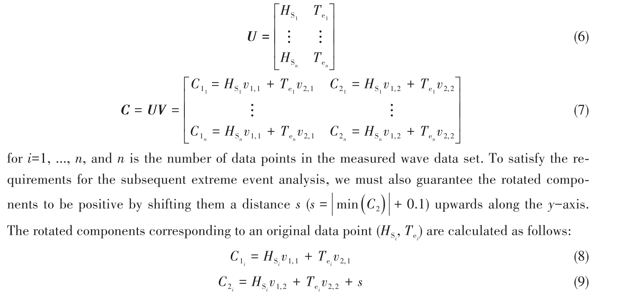
whereC1iis theith rotated first component corresponding to anith original significant wave height data pointHSiand anith original energy period data pointTei,C2iis theith rotated second component corresponding to anith original significant wave height data pointHSiand anith original energy period data pointTei,sis a shifting distance.By utilizing the following two equations, we can transform the point (C1i,C2i) in the principal component space back to the corresponding point in the original input space:

After rotating the input variables into the principal component space,we can fit the cumulative distribution function ofC1with an inverse Gaussian distribution:

whereΦ( )is the standard Gaussian distribution function, andμandλare the location and scale of the inverse Gaussian distribution respectively.In Eq.(12)xstands forC1.In probability theory,the inverse Gaussian distribution (also known as the Wald distribution)is a two-parameter family of continuous probability distributions.The inverse Gaussian distribution has several properties analogous to a Gaussian distribution.The name can be misleading: it is an‘inverse’only in that, while the Gaussian describes a Brownian motion's level at a fixed time, the inverse Gaussian describes the distribution of the time of a Brownian motion with positive drift takes to reach a fixed positive level.Its cumulant generating function (logarithm of the characteristic function)is the inverse of the cumulant generating function of a Gaussian random variable.

The values ofC2are sorted according to their correspondingC1values and split into bins.The parameters of theC2distributions are fit as functions of the representative value ofC1for each bin in order to represent the dependency betweenC1andC2that has not yet been captured.Based on the shape of the cumulative distribution functions for each bin ofC2, a Gaussian distribution expressed as follows is chosen to fit each CDF ofC2:

whereerfis the error function,and the meanμand the standard deviationσare the parameters defining the Gaussian distribution.In the following we will use a simple linear approximation to fitμas a function ofC1.Furthermore, we will use a constrained quadratic approximation to fitσas shown in Eqs.(15)-(17):

As soon as the sun rose the King came, and when he perceived the gold he was astonished and delighted, but his heart only lusted more than ever after the precious metal

In the following we call the procedures in this section for obtaining theq-probability environmental contour lines the PCA-IFORM environmental contour method.Robertson et al[10]performed the holistic marine energy resource assessments from a wave and offshore wind perspective of metocean conditions.In their research they generated accurate environmental contours using the WDRT toolbox[11]based on the PCA-IFORM environmental contour method.Li and Zhang[12]conducted long-term fatigue damage assessment for a floating offshore wind turbine under realistic environmental conditions.They pointed out that building an accurate environmental model that could accurately describe the multivariate dependence among environmental parameters is essential to ensure structural lifetime safety and reliability,and they particularly mentioned that the PCA-IFORM environmental contour statistical model could be used to achieve this objective.Yang et al[13]studied the characteristics and variability of the nearshore wave resource on the U.S.West Coast.They pointed out that environmental contours are widely used in the maritime industry for design,including the design of wave energy converters.Taking advantage of the long-term hindcast data set,environmental contours were computed by them at the four study locations using the PCA-IFORM environmental contour method as described by Eckert-Gallup et al[9].They found that the wave heights corresponding to the 100-year event(1%yearly probably of occurrence)decrease with latitude.Coe et al[14]performed a full long-term design response analysis of a wave energy converter.Environmental characterization and selection of sea states for this analysis at the intended deployment site were performed using principle-components analysis.Sea states for full long-term analyses in this study were obtained using a modified inverse first-order reliability (I-FORM) method (i.e., PCA-IFORM environmental contour method).This process was conducted using the tools provided in the WEC Design Response Toolbox(WDRT)[11].Finally,Coe et al[15]carried out a classical survey of WEC reliability, survival and design practices.In their paper they pointed out that‘An improved version of the I-FORM process is presented in Ref.[9].Here, a principle component analysis (PCA) approach is applied to better utilize the physical relationship between wave period and height.’.

2 Theories for simulating nonlinear random waves

In a classical paper[16]regarding estimating the extreme structural dynamic responses of offshore structures based upon the environmental contour method, the authors pointed out that‘The worst sea state turns out to be the highest sea state along the contour.’.After the highest sea state is identified along the PCA- IFORM (or Rosenblatt-IFORM) environmental contour, we can simulate nonlinear wave surface elevations based on the data of this highest sea state according to the following theories:

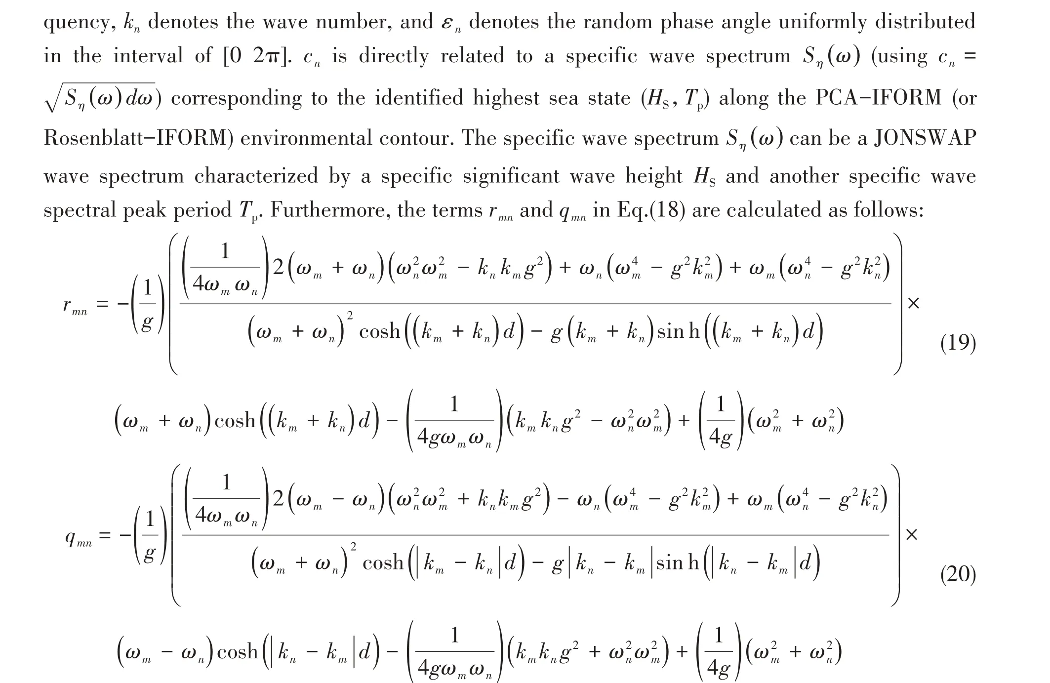
wheredis the water depth.

3 Environmental contours calculation examples based on the measured data at National Data Buoy Center(NDBC)Station 42012

Fig.2 shows the 50-year environmental contours generated by the PCA-IFORM method and the Rosenblatt-IFORM method for NDBC.The red‘points’in Fig.2 show the measured data for the NDBC station 42012.The solid blue line in Fig.2 represents the 50-year environmental contour generated using the Rosenblatt-IFORM environmental contour method.We can

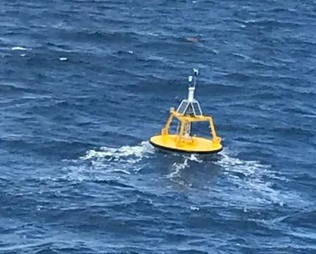
Fig.1 Buoy of the NDBC Station 42012

In this chapter we will present our environmental contours calculation examples based on the measured data at NDBC Station 42012.This buoy is installed at Orange Beach-44 nautical miles southeast of Mobile, AL, U.S.A.The water depth at this location is 25.9 m.Fig.1 shows the buoy of the NDBC Station 42012.In the following we will use the PCA- IFORM method and the Rosenblatt-IFORM method to generate environmental contours based on the 86089 hourly observations ofHSandTptaken from Jan.1, 2009 to Dec.31, 2019 at NDBC Station 42012.clearly find that this 50-year solid blue contour does not include all of the measured NDBC 42012 data of about 11 years.Furthermore, this solid blue contour does not follow the shape of trends of the measured NDBC 42012 data either.This solid blue contour fails for coverage in the area where theHSvalues are very high.These calculation results demonstrate that the obtained Rosenblatt-IFORM environmental contour does not have good predictivity.

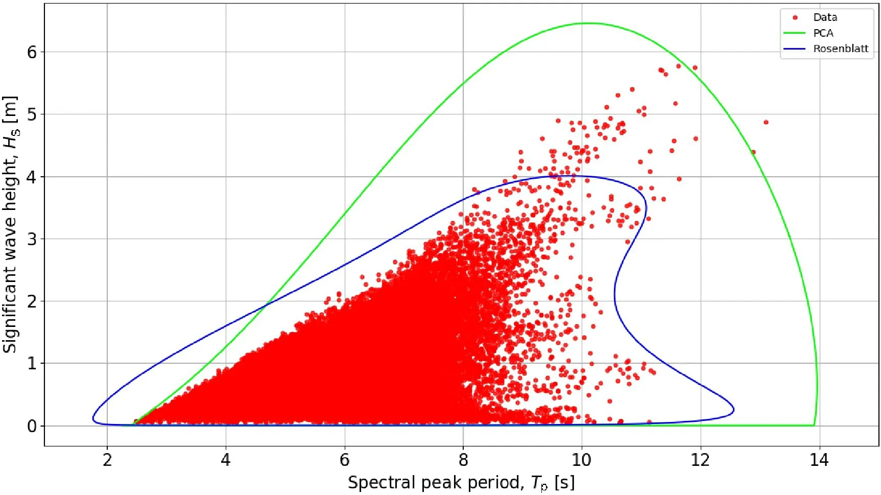
Fig.2 50-year environmental contours created by the PCA-IFORM method and the Rosenblatt-IFORM method for NDBC 42012

The solid green curve in Fig.2 shows the 50-year environmental contour generated by using the PCA-IFORM method.We can clearly find that this solid green curve fit quite well with both higher and smaller values ofHS.We can also clearly notice that this solid green curve does include most of the measured NDBC 42012 data, missing only three data points.Furthermore, this solid green curve also follows quite well the shape of trends of the measured NDBC 42012 data.This solid green curve is very successful for coverage in the area where theHSvalues are very high.These calculation results indicate that the environmental contour generated using the PCA-IFORM method does have good predictivity.

4 Extreme structural dynamic responses of a 5 MW offshore wind turbine

4.1 Chosen 5 MW offshore wind turbine

In the following we will calculate the extreme structural dynamic responses of the NREL (National Renewable Energy Laboratory) 5 MW monopilesupported offshore wind turbine (as shown in Fig.3)based on the theoretical methods as illustrated in Chapter 1 and Chapter 2.This chosen offshore wind turbine system is composed of a 5 MW wind turbine, a tower and a monopile foundation[17].The NREL 5MW baseline offshore wind turbine has three blades.The rotor diameter is 126 m and the hub diameter is 3 m.The rotor mass is 110 000 kg, and the nacelle mass is 240 000 kg.The NREL 5 MW fixed-bottom monopile wind turbine is sited at a water depth of 25.9 m.At the seabed mudline, the tower attaches to the monopile foundation of the same dimensions (with an outer diameter of 6 m and a wall thickness of 6 cm).The foundation is embedded 36 m into the seabed.The hub height of the wind turbine is 84.1 m from the mean sea water line.The draft of this offshore wind turbine is 25.9 m.These detailed properties and dimensions of this offshore wind turbine system is also contained in Re.[17].

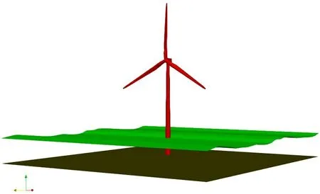
Fig.3 NREL 5 MW monopile-supported offshore wind turbine system

4.2 Calculation examples

From Fig.2 (50-year environmental contours created by the PCA-IFORM method and the Rosenblatt-IFORM method for NDBC 42012) we can find that in the highest sea state (50 years of extreme sea conditions) along the PCA-IFORM environmental contour,HS=6.47 m andTp=10.16 s.We can also find that in the highest sea state (50 years of extreme sea conditions)along the Rosenblatt-IFORM environmental contour,HS=4.03 m andTp=9.87 s.In the following calculation examples,the aforementioned NREL 5 MW offshore wind turbine is assumed to be installed at a site with an IEC (International Electrotechnical Commission) Class I-B wind regime.The turbulence wind random field over the turbine rotor plane is simulated using the computer code TurbSim with a wind speed of 1.6 m/s at the hub height.

The structural dynamic responses of the aforementioned NREL 5 MW offshore wind turbine have been calculated by implementing time domain simulations in FAST.Hydrodynamic loads acting on the offshore wind turbine support structure are computed by applying Morison's equation.The nonlinear random ocean waves have been simulated using the theories in Chapter 2 based on a JONSWAP wave spectrum with a significant wave height of 6.47 m and a spectral peak period of 10.16 s.For this highest sea state along the PCA-IFORM environmental contour in Fig.2, we have imple-mented six 10 min stochastic time domain simulations.Tab.1 shows the first and second random seeds of incident waves during these six simulations.Fig.4 shows one simulated 10 min time series of the fore-aft shear forces at the mudline of the offshore wind turbine.In our study we have joined the aforementioned six 10 min time series into one and tried to forecast the 50-year extreme shear force based on this joint one series by using the peaks-over-threshold method[18-20].

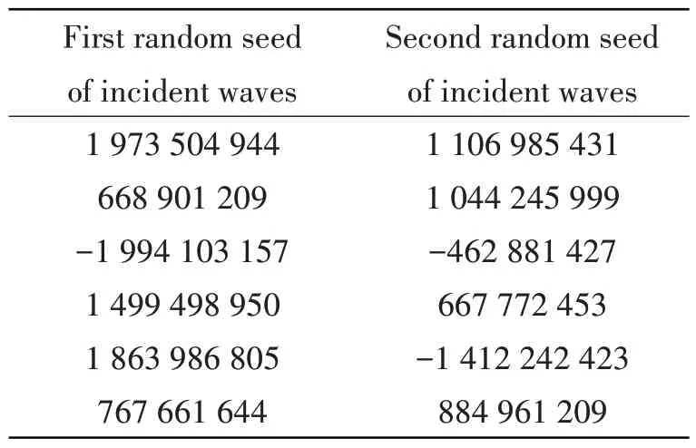
Tab.1 1st and 2nd random seeds of incident waves during 6 simulations(PCA-IFORM case)

Fig.4 One simulated 10 min time series of the fore-aft shear forces at the mudline of the offshore wind turbine

For the joint 60 min time series of the foreaft shear forces at the mudline of the offshore wind turbine we have obtained an optimal threshold level of 2 334 500 N as shown by the green vertical line in the mean excess plot (i.e.,Fig.5).We have extracted 18 local extremes from the aforementioned time series above the threshold level of 2 334 500 N and fitted a Generalized Pareto distribution as shown by the solid green line in Fig.6 using the maximum likelihood method.In Fig.6,the blue straight lines are the empirical distribution (histogram) obtained from these extracted 18 local extremes.We can find that the fitted Generalized Pareto distribution fits the empirical distribution (histogram) very well.The two red dashed curves in Fig.6 are the upper and lower 95%confidence interval lines respectively.

In this study we want to predict the 50-year extreme structural dynamic responses of the NREL 5 MW monopile-supported wind turbine.That is to say, our aimed exceedance probability target is 2×10-2.As pointed out in the theory of the environmental contour method in Ref.[8]:‘The fractile level,p, will depend on the aimed exceedance probability target,q, …… For most practical systems,p=0.90 seems reasonable forq=10-2, whilep=0.95 may be more adequate forq=10-4.’.Therefore,it is reasonable for us to choosep=0.85 because our aimed exceedance probability target is 2×10-2.Consequently, based on the aforementioned fitted Generalized Pareto distribution we finally obtain that the 0.85 fractile level load (fore-aft shear force at the mudline) is 2.922 2E+06 N, and this number is summarized in Tab.3.Other data in Tab.3 have been obtained in a similar manner.

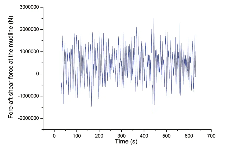
Fig.5 Mean excess plot for the fore-aft shear forces at the mudline of the offshore wind turbine

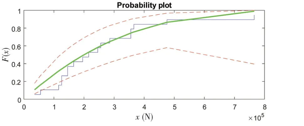
Fig.6 Fitted generalized Pareto distribution as shown by the solid green line

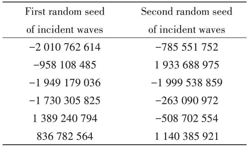
Tab.2 1st and 2nd random seeds of incident waves during 6 simulations(Rosenblatt-IFORM case)

Here we should further explain the calculation processes for obtaining the data in Column 3 of Tab.3, i.e., the calculation results based on the extreme sea state (HS=4.03 m andTp=9.87 s) obtained using the Rosenblatt-IFORM environmental contour method.For this highest sea state along the environmental contour based on the Rosenblatt-IFORM contour method, we have also carried out six 10 min stochastic time domain simulations.Tab.2 shows the first and second random seeds of incident waves during these six simulations.Subsequently, using the similar procedures for obtaining the fore-aft shear force result list in Column 2 of Tab.3 we have finally obtained the data as listed in Column 3 of Tab.3.

Tab.3 50-year extreme response values based on 50-year extreme sea states obtained using different methods

By carefully studying the calculation results listed in Tab.3 we can find that the 50-year extreme fore-aft shear force value based on the 50-year extreme sea state obtained using the PCA-IFORM contour method is 27.6% larger than the corresponding value obtained based on the Rosenblatt-IFORM contour method.The 50-year extreme fore-aft bending moment at the mudline based on the extreme sea state obtained using the PCA-IFORM contour method is 10.6% larger than the corresponding value obtained based on the Rosenblatt-IFORM contour method.Because we have already demonstrated in Chapter 3 that the PCA-IFORM contour method can generate more accurate and realistic environmental contours than the Rosenblatt-IFORM contour method,the 50-year extreme responses(fore-aft shear force and bending moment at the mudline)predicted based on the 50-year extreme sea state obtained using the PCA-IFORM contour method are undoubtfully more accurate.This means that an offshore wind turbine design based on the extreme dynamic response values predicted using the highest sea state data along a PCA-IFORM contour will be safer.On the contrary, structural failures will likely occur for an offshore wind turbine design when the input extreme sea state is forecasted using the Rosenblatt-IFORM environmental contour method.

5 Concluding remarks

In order to overcome the shortcomings of the traditional Rosenblatt-IFORM environmental contour method, the use of the PCA-IFORM contour method for generating more accurate environmental contours was proposed.Based on the measured data at a chosen offshore site, it was demonstrated that the PCA-IFORM contour method can generate more accurate and realistic environmental contours than the Rosenblatt-IFORM environmental contour method.The 50-year extreme structural dynamic responses of a monopile-supported 5 MW offshore wind turbine installed at this chosen offshore site were calculated based on the PCA-IFORM contour method and the traditional Rosenblatt-IFORM environmental contour method.It is concluded that an offshore wind turbine design based on the extreme dynamic response values predicted by using the highest sea state data along a PCA-IFORM contour will be safer while an offshore wind turbine design will likely result in structural failures when the input extreme sea state is forecasted using the Rosenblatt-IFORM environmental contour method.In summary, this study highlights the necessity and importance of using more realistic environmental contours (such as those generated using the PCA-IFORM contour method)in prediction of the extreme structural dynamic responses of offshore wind turbines.