Artificial neural network algorithm for pulse shape discrimination in 2πα and 2πβ particle surface emission rate measurements

Yuan‑Qiao Li · Bao‑Ji Zhu,2 · Yang Lv · Heng Zhu,2 · Min Lin,2 · Ke‑Sheng Chen,2 · Li‑Jun Xu,2

Abstract To enhance the accuracy of 2πα and 2πβ particle surface emission rate measurements and address the identification issues of nuclides in conventional methods, this study introduces two artificial neural network (ANN) algorithms: back-propagation(BP) and genetic algorithm-based back-propagation (GA-BP).These algorithms classify pulse signals from distinct α and β particles.Their discrimination efficacy is assessed by simulating standard pulse signals and those produced by contaminated sources, mixing α and β particles within the detector.This study initially showcases energy spectrum measurement outcomes,subsequently tests the ANNs on the measurement and validation datasets, and contrasts the pulse shape discrimination efficacy of both algorithms.Experimental findings reveal that the proportional counter’s energy resolution is not ideal, thus rendering energy analysis insufficient for distinguishing between 2πα and 2πβ particles.The BP neural network realizes approximately 99% accuracy for 2πα particles and approximately 95% for 2πβ particles, thus surpassing the GA-BP’s performance.Additionally, the results suggest enhancing β particle discrimination accuracy by increasing the digital acquisition card’s threshold lower limit.This study offers an advanced solution for the 2πα and 2πβ surface emission rate measurement method, presenting superior adaptability and scalability over conventional techniques.

Keywords Pulse shape discrimination · Artificial neural networks · Alpha and beta sources · Multi-wire proportional counter · Surface emission rate

1 Introduction

According to international and Chinese standards [1–4],αandβplane sources are essential for calibrating, verifying, and ensuring the stability of radioactivity measurement and surface contamination monitoring instruments.In international comparisons [5], most institutions utilize a gas-flow 2π multi-wire proportional counter as the detector for 2παand 2πβparticle measurements, offering a detection efficiency of almost 100% for these particles.However, owing to the multi-wire proportional counter’s low energy resolution, discriminating between particles becomes challenging.Some institutions[6–8] continue using the single-channel pulse amplitude analysis method for counting, which measures pulse amplitude but fails to discriminate the pulse shapes of varying radio-nuclides.With the rapid advancement of digital signal acquisition technology, some establishments [9] have realized plane-source spectrum measurements.Nonetheless, owing to varying plane source preparation processes, uncertainty regarding the spectral consistency of the same radionuclide exists.Moreover, for contaminated detectors or mixed plane sources infused with other radio-nuclides, the conventional 2π multi-wire proportional counter cannot identify radioactive particles or assess plane source purity.Historically,αandβparticle discrimination necessitated a blend of energy, time, and frequency analysis techniques.This poses challenges when measuring beta particles in a detector contaminated by alpha particles.The increased operating voltage results in the ionization effect of alpha particles to enter the limited proportional region.Consequently, the collected ionization numberNdoes not align proportionally with the initial total ionizationN0, thereby leading to a spike in detector counts.Thus, enhancing the accuracy of 2παand 2πβsurface emission rate measurements demands effective particle discrimination.

Various particle-identification models have been developed over the past four decades.Pulse shape discrimination (PSD)techniques can be classified into three main categories: time domain, frequency domain, and machine learning.These methods are listed in Table 1.

Discrimination techniques for particles based on time- or frequency-domain attributes and fuzzy C-mean clustering [10]utilize limited features of the pulse shape for classification.Such methods may overlook other significant pulse signal features.Although they exhibit effective discrimination, these techniques consume significant processing time for multi-particle classification, thus compromising efficiency.The artificial neural network (ANN) approach offers automatic learning and parameter adjustment capabilities, thus reducing labor and time expenditure.This method can expand the radio-nuclide classification with fresh training data, thus enhancing system scalability and adaptability.

ANNs have been employed for nuclear pulse shape analysis [11, 12]; however, initial applications were constrained by inadequate computational power, limited input parameters, few training samples, and a low ADC sampling rate.Over the past decade, ANN methodologies have evolved, finding successful application inγparticle-specific activity measurements [13],α/γidentification [14],n/γpulse shape discrimination [15–19],γ-energy spectrum analysis [20–22], and pulse shape repair[23–26].However, most studies focused on semiconductor and scintillator detectors, with ANNs not yet applied to 2παand 2πβparticle surface emission rate measurements.

The objective of the current study is to introduce two ANN algorithms for the discrimination of 2παand 2πβparticles.Neural network methods are employed to distinguish pulse signals adulterated by non-standard ionized particles within a simulated environment, considering the detector’s dual standard-voltage operational states.The study examines the viability of this technique for surface emission rate measurement systems reliant on 2π multi-wire proportional counters.Furthermore, it discusses the efficacy of different neural network architectures and algorithmic parameters.The study initially details the experimental setup, training dataset, and validation set.Subsequently, it elucidates the characteristics of the two ANNs and offers an in-depth overview of their application.Finally, the findings derived from the experimental data concerning both ANNs are presented.

2 Experimental setup

2.1 Data acquisition methods

In this study, the detector employed was a large-area 2π multi-wire proportional counter [27], a product of the China Institute of Atomic Energy (CIAE).The detector operates at voltages of 2100 V forαsources and 2800 V forβsources.It boasts a counting response uniformity exceeding ± 0.4%, an effective detection area of approximately 1400 cm2, shortterm stability measurements surpassing 0.3% over 8 h, and long-term stability measurements surpassing 0.8% over a year.A schematic of the 2π multi-wire proportional counter system used in this study is shown in Fig.1.The counter utilized P-10 gas for counting, composed of 90% Ar and 10%CH4.The gas flow rate was consistently held at 20–60 mL/min during the detector’s routine operation.All sources deployed in the experiments were calibrated, with their traces leading back to the 2παand 2πβsurface emission rate standard devices at CIAE.To align the count rate recorded by the digital acquisition card with the plane sources’ surface emission rate, the acquisition card’s pulse amplitude trigger threshold was adjusted during the surface emission rate calibration experiments.For configuring the acquisition card, a fixed sampling length was determined based on the pulse’s maximum width.A pertinent starting point for sampling was selected.Amplitude and time resolutions were fine-tuned to prevent signal saturation and to ensure comprehensive pulse signal capture across all plane source varieties.Each signal sample spanned 1048 ns, with a time step of 1 ns, and it was divided into 1048 equidistant components.This type of configurations implied that minimal saturation or signal pile-up was observed throughout data collection.The digital acquisition card was then primed to yield an energy spectrum, which is elaborated in Sect.4.1.

Fig.1 Block diagram for pulse signal acquisition for large area flowthrough 2π multi-wire proportional counter

Table 1 Classification of particle pulse shape discrimination techniques

2.2 Training and verification datasets

In this study, twoαplane sources (238Pu and241Am) and twoβplane sources (204Tl and90Sr) were employed for the experiments.The chosenα-sources,241Am and238Pu, are prominent in 2π surface emission rate measurements owing to their high purity relative to otherα-plane sources.Additionally, the high-energyβ-sources,204Tl and90Sr, were selected to minimize noise interference and to facilitate neural network training with broader and more pronounced pulse shapes for effective classification.Six distinct sets of pulse measurements were acquired, with each set comprising signals from a sole radiation source.Four of these sets captured measurements of 2παand 2πβsurface emission rates under standard conditions.The remaining two sets simulated signals contaminated by extraneous particles.To represent particle discrimination and surface emission rate measurements in real-world scenarios, the data were categorized into a 2παmeasurement dataset and 2πβmeasurement dataset.The 2παmeasurement dataset encompassedα1,α2, andα3.Specifically,α1andα2correspond to pulse shapes obtained from the detector for238Pu and241Am, both at a direct current (DC) voltage of 2100 V.Whereasα3contains pulse shape data from the204Tl source, also at 2100 V DC, simulating the pulse data acquired duringβparticle contamination in 2παsurface emission rate measurements.The 2πβmeasurement dataset encompassedβ1,β2, andβ3.Theβ1andβ2subsets contain pulse shapes from the detector for204Tl and90Sr, measured at a DC voltage of 2800 V.Whereas theβ3subset contains pulse shape data from the241Am source at 2800 V DC, emulating the pulse data influenced byαparticle contamination in 2πβsurface emission rate measurements (Tables 2 and 3).

The204Tl source was consistent inα3andβ1datasets,whereas the241Am source was utilized inα2andβ3sets.The pulse sample count for theα3dataset was limited.This was because the204Tl operated at a DC voltage of 2100 V, falling beneath the ionization threshold.Hence, the mostly signal captured was the detector’s background signal.

Table 2 2πα experimental dataset

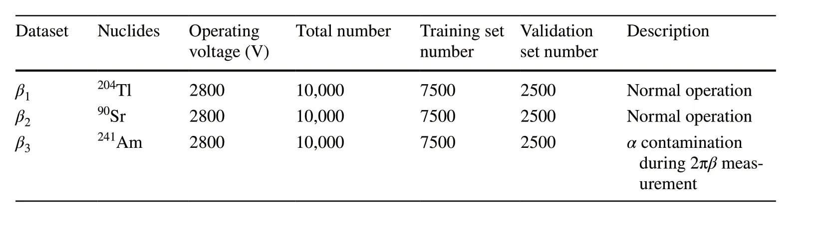
Table 3 2πβ experimental dataset

Fig.2 Typical structural model of a neural network.(Color figure online)

3 Artificial neural network

The structure of the artificial neural network consists of an input layer, a hidden layer, and an output layer, as illustrated in Fig.2.In this structure, “x” represents the input signal.Each neuron within the network receives input signals from preceding neurons.These signals traverse connections characterized by weights (w1,w2) and biases (b1,b2).The neuron then aggregates these to derive a total input value.Subsequently, this value is compared with the neuron’s threshold value and processed through an activation function.The resultant output is forwarded as input to neurons in the subsequent layers.

This study applied two different neural network algorithms for 2παand 2πβpulse shape classification prediction:back-propagation (BP) and genetic algorithm-based backpropagation (GA-BP).This section describes the principles,network structures, and parameters of the algorithms.Both algorithms were implemented in MATLAB (MathWorks,Natick, MA, USA).The computational hardware for the BP neural network comprised a CPU (Intel i5-12400F) with 16 GB of RAM, and that for the GA-BP neural network comprised a CPU (Intel i9-12900 K) with 16 GB of RAM.

3.1 BP neural network

3.1.1 Principle

A BP neural network serves as the fundamental element of a feed-forward network.With its straightforward architecture, numerous tunable parameters, and robust operability, it stands as the most prevalent and advanced training algorithm.The neural network’s design encompasses the count of neurons in the input, hidden, and output layers.Initial training parameters encompass the learning rate, maximum iteration count, number of validation failures, interlayer activation functions, evaluation function, and its minimal value.The error, which is the discrepancy between the output layer’s outcome and actual result matching the input data, is the back-propagated information.With each forward and backward propagation, the neural network updates its parameters.Training entails repeated forward and backward propagations, which refine their parameters to approximate a genuine relationship.In theory, a sufficiently layered and node-equipped network can approximate any nonlinear functional relationship.

3.1.2 Network structure and parameters

The same BP neural network was trained on two datasets:2παand 2πβ.Each dataset encompassed three pulse types(α1,α2, andα3for 2παandβ1,β2, andβ3for 2πβ).The network featured 1048 input neurons, correlating with the amplitude vector of a singular pulse on a continuous time axis, and three output neurons representing the pulse types.The MATLAB function vec2ind was employed to inversely normalize and categorize the output neurons.For the 2παdataset, the classification results were defined as follows.

whereas for the 2πβdataset, the classification results were defined as follows.

A sigmoid function was used as the activation function for our back-propagation neural network.This function maps the weighted sum of the neurons,x, to a value between 0 and 1, effectively capturing the nonlinearity of the input signal.

The performance of our back-propagation neural network was evaluated using mean square error (MSE), which measures how well the model’s predictionŶmatches the true labelY.Specifically, MSE can be applied to both linear regression and simple classification problems.It is expressed as follows.

Table 4 BP neural network structure parameters

Fig.3 Block diagram of a BP neural network system with one hidden layer

Four BP neural network models with varying numbers of hidden layers and neurons were analyzed.The ideal count of hidden layers and neurons often lacks a definitive benchmark and is usually identified through experimentation.Although more hidden layers and neurons can enhance the model’s fitting capacity, they may also lead to overfitting and pose challenges during training.Models 1 and 2 incorporate a single hidden layer, whereas Models 3 and 4 encompass two hidden layers.The number of neurons in each hidden layer was adjusted to assess its impact on prediction outcomes.The specifications of the network structure are listed in Table 4 and are further elaborated upon in Results section.A schematic of the neural network system for Models 1 and 2 is illustrated in Fig.3.

Based on prior experience, the learning rate, maximum number of iterations, count of validation failures,and minimum threshold of the performance indexεwere determined.To satisfy the criteria for performance and gradient, the maximum iteration count should be suffi-ciently high.Generally, the count of validation failures falls between 10 and 20.Thus, herein, a threshold ofε= 1 × 10–6was adopted as the minimum performance index value.

3.2 GA-BP Neural networks

3.2.1 Principle

Although BP neural networks are widely prevalent, they present challenges such as languid convergence, susceptibility to local minima, and indeterminate network structures.To enhance these attributes, this study employed genetic algorithms for the optimization of the neural networks.Serving as models of biological evolution, genetic algorithms mimic processes of natural selection and genetic inheritance.In the 1960s, Holland introduced a mathematical representation of these algorithms [28, 29].This method models the problemsolving approach, akin to biological evolution, essentially encompassing the crossover and mutation [30–32] of genetic elements.In this study, genetic algorithms were applied to determine superior initial parameters during forward propagation, which were subsequently refined using back-propagation.Figure 4 illustrates a layout of the genetic algorithmenhanced back-propagation (GA-BP) neural network.Once the structure of the BP neural network was confirmed, its weight and bias parameters were transcribed as elements of chromosomes within the genetic realm.This step enabled the creation of an initial chromosome assembly.Each chromosome was subsequently translated back into a neural network, where its output and error metrics were discerned through forward computations and back-propagation using training datasets.Subsequently, fitness scores for every chromosome were assessed based on the error metrics or alternative measures.An apt fitness function was then engaged to evaluate the viability of each chromosome in the collective.A selection of the most promising chromosomes,as determined by their fitness scores, was advanced to the succeeding generation.Before assembling a new generation,crossover and mutation procedures augmented the genetic diversity of the group.Following a set number of cycles, the chromosome with the foremost fitness score was adopted as the concluding outcome.The processes of population initialization, chromosome inheritance, crossover, and mutation are depicted in Fig.5.

Fig.4 Schematic of a genetic algorithm-based neural network (GABP)

3.2.2 Network structure and parameters

An identical GA-BP neural network was employed to train with the 2παand 2πβmeasurement datasets.Parameters from Model 1 of the BP neural network informed the configuration of the input layer, hidden layer, output layer, activation function, performance evaluation index, learning rate,maximum iteration count, and number of validation failures.For the genetic algorithm, the parameters encompassed population size, number of genetic generations, and the choices of an appropriate fitness function, selection function, and crossover function.

Three distinct GA-BP neural network structures, each with varied genetic algorithm parameters, are crafted as detailed in Table 5.Models 5 and 6 differ in terms of their number of generations, whereas Models 5 and 7 differ in terms of their population size.A detailed comparison of these models, rooted in their training outcomes, is elaborated upon in Sect.4.

Genetic algorithm functions were implemented using MATLAB’s GAOT toolbox.The fitness function was gabpEval, selection function was normGeomSelect (geometric ranking selection), crossover function was arithXover(arithmetic crossover), and mutation function was nonUnifMutation (non-uniform mutation).Default parameters were maintained for these functions.

4 Result

Herein, the energy spectrum measurements of plane sources were obtained and the two ANNs methods for identifying 2παand 2πβparticles were compared.

4.1 Results of energy spectrum measurements

The energy spectra of the four-plane sources were measured using the experimental equipment described in this study.

The energy spectra of238Pu and241Am used in this study are shown in Fig.6.The proportional counter exhibited a low energy resolution, and the particle energies of238Pu and241Am ranged from 300 to 2500 and from 600 to 3500 channel sites, respectively.Nuclide particles could not be identified in the channel address range of 600–2500.Identification was possible with single-nuclide measurements but not with mixed measurements.

Fig.5 Population initialization and chromosome inheritance, crossover, and mutation processes in genetic algorithms.(Color figure online)

Table 5 GA-BP neural network structure and genetic algorithm parameters

Fig.6 Energy spectra of a 238Pu and b 241Am with a cumulative measurement time of approximately 10 s

Figure 7 shows the energy spectra of the two-plane sources.The spectra overlapped considerably and were difficult to analyze.Only a few particles that were not in the energy-crossing region were identified.

4.2 Results of BP neural network training

Four BP neural network models were trained using randomized data arrangements from 2παand 2πβexperimental datasets.The results for the four network structures are presented in Table 6.

A comparison of pulse shape discrimination results for 2παand 2πβparticles using four BP neural network models reveals that Model 4 exhibited the highest accuracy for the training and validation sets, as well as the linear regression coefficient.The confusion matrix results of the 2παparticle training and validation sets of Model 4 are shown in Fig.8,and the confusion matrix results of the 2πβparticle training and validation sets of Model 4 are shown in Fig.9.

Fig.7 Energy spectra of a 204Tl and b 90Sr with a cumulative measurement time of approximately 10 s

Table 6 Pulse shape discrimination results for 2πα and 2πβ particles using BP neural network model

Fig.8 Confusion matrix for 2πα dataset using BP neural network(Model 4): a training dataset and b validation dataset.The matrix has three rows and three columns; each row represents the classification results of true values for α1, α2, and α3 datasets, and each column represents the classification results of predicted values for α1, α2, and α3 datasets.Here,1, 2, and 3 denote α1, α2, and α3 datasets, respectively.(Color figure online)

4.3 Results of GA-BP neural network training

Three GA-BP models were employed to train 2παand 2πβexperimental datasets.The data arrangements for both datasets were randomized.The results for the three network structures are presented in Table 7.

Fig.9 Confusion matrix for 2πβ dataset using BP neural network (Model 4): a training dataset and b validation dataset.The matrix has three rows and three columns; the rows and columns represent the true value classification results and predicted value classification results, respectively.Here, 1,2, and 3 denote β1, β2, and β3 datasets, respectively.(Color figure online)

Table 7 Pulse shape discrimination results for 2πα and 2πβ particles using GA-BP neural network model

Fig.10 Confusion matrix for 2πβ dataset using GA-BP neural network (Model 7): a training dataset and b validation dataset.The matrix has three rows and three columns; the rows and columns represent the true value classification results and predicted value classification results, respectively.Here, 1,2, and 3 denote α1, α2, and α3 datasets, respectively.(Color figure online)

Fig.11 Confusion matrix for 2πβ dataset using GA-BP neural network (Model 7): a training dataset and b validation dataset.The matrix has three rows and three columns; the rows and columns represent the true value classification results and predicted value classification results, respectively.Here, 1,2, and 3 denote β1, β2, and β3 datasets, respectively.(Color figure online)

A comparison of pulse shape discrimination results for 2παand 2πβparticles using three GA-BP neural network models reveals that Model 7 exhibited the highest accuracy for the training and validation sets, as well as the linear regression coefficient.The confusion matrix results of the 2παparticle training and validation sets of Model 7 are shown in Fig.10,and the confusion matrix results of the 2πβparticle training and validation sets of Model 7 are shown in Fig.11.

5 Discussion

The energy spectrum measurements detailed in Sect.4.1 indicate that relying solely on energy analysis techniques is an ineffective strategy for distinguishing between 2παand 2πβparticles.To accurately differentiate between pulse signals, the energy analysis should be combined with information on the signal timing and frequency.Nonetheless, merging these methods necessitates more resources and time, thus compromising efficiency.

Evidently from the results showcased in Tables 6 and 7, several BP neural network models generally surpass the GA-BP neural network models in terms of accuracy rates and linear regression coefficients.Importantly, the BP neural network models not only demonstrated superior outcomes but also necessitated shorter training durations, particularly when the computing resources (CPU) were relatively poor.

The performance in distinguishing 2παparticles is illustrated in the confusion matrices depicted in Figs.8 and 10.Figures 8a, b highlight Model 4’s high prediction accuracy,as all three 2παsignals surpassed 99%.Conversely, the accuracy rates for training and validation sets using Model 7 were somewhat subpar.Figure 10b indicates that 112 pulse shapes from theα1set were incorrectly identified asα2; consequently, the accuracy rate was approximately 95.5%.This suggests that Model 7 is more prone to misclassifyingα1signals asα2.Hence, the BP neural networks were significantly more effective in distinguishing 2παparticles.

With respect to the discrimination of 2πβparticles, the corresponding confusion matrices are outlined in Fig.9 and 11.Forβ1, both neural network algorithms showcased exceptional classification, with Fig.9b projecting a 99.4%accuracy for theβ1validation set.An analysis of the predictive classifications in the matrix to understand the suboptimal discrimination shows that the predicted outcomes forβ1andβ2datasets are commendable, thereby discounting the prospect of a high detector background signal.Thus, the poor classification ofβ2andβ3datasets can be attributed to the resemblance of pulse shapes in theβ2dataset to those in theβ3dataset, thus leading to decreased accuracy for the overall dataset.The introduction ofα-nuclide (241Am) contamination to the detector made it more likely to misidentify contaminated signals as belonging to theβ2dataset.Observations of theβ3set via an oscilloscope revealed that signals in theβ3dataset mainly consisted of low-energy pulses,suggesting that the pulse signals ofαat a high voltage of 2800 V are resemblance to the signals ofβof low energy.Future research could focus on establishing an apt energy threshold to filter these low-energy signals using a digital acquisition card, followed by estimating the 2πβsurface emission rate post a minor energy adjustment.

6 Conclusion

In this study, two neural network-driven pulse shape discrimination methods were developed to address the challenges inherent in traditional 2παand 2πβparticle surface emission rate measurements.These techniques were assessed over six distinct datasets, where four were under standard operation and two simulated contamination scenarios.Various network architectures and parameters were explored for both methodologies, with the optimal parameters being determined based on empirical findings.

The results demonstrated the potential of neural network algorithms in distinguishing particle types in radionuclide-contaminated detectors.Following successful classification, surface emission rate measurements can be derived from a statistical analysis, thus enabling more detailed nuclide mixture assessments.However, a notable challenge emerged: the absence of a universally accepted criterion for tuning neural network algorithm parameters.This necessitated adjustments based on hands-on experiments or expert recommendations.

When comparing the two algorithms, the BP neural network exhibited superior efficiency in the training process than the GA-BP neural network.The intricacies associated with the parameter requirements of the latter may account for this discrepancy.If these parameters are not set properly, then it could initiate an exhaustive series of iterative computations, potentially causing the network to prematurely converge or become ensnared in a local optimum.

For more accurate 2πβparticle surface emission rate assessments and nuclide identification, we suggest an adjustment to the energy threshold of the digital acquisition system.This would ensure the extraction of a more refined training dataset.

In summation, the study highlighted the efficacy of neural networks in 2παand 2πβpulse shape discrimination and subsequent classification for particle surface emission rate evaluations.This approach eliminates the need for signal preprocessing and significantly enhances pulse shape differentiation efficiency.Furthermore, its inherent adaptability and scalability hint at its potential applicability in otherαandβdetection mechanisms.

Author contributionsAll authors contributed to the study conception and design.Material preparation was performed by Yuan-Qiao Li,Min Lin, and Ke-Sheng Chen, data collection was performed by Yuan-Qiao Li, Bao-Ji Zhu, and Heng Zhu, analysis was performed by Yuan-Qiao Li, Min Lin, and Li-Jun Xu.The first draft of the manuscript was written by Yuan-Qiao Li and Yang Lv; all authors commented on previous versions of the manuscript.All authors read and approved the final manuscript.

Data availabilityThe data that support the findings of this study are openly available in Science Data Bank at https:// www.doi.org/ 10.57760/ scien cedb.j00186.00206 and https:// cstr.cn/ 31253.11.scien cedb.j00186.00206.

Declarations

Conflict of interestThe authors declare that they have no competing interests.