A discrete Boltzmann model with symmetric velocity discretization for compressible flow

Chuandong Lin(林传栋), Xiaopeng Sun(孙笑朋), Xianli Su(苏咸利),Huilin Lai(赖惠林), and Xiao Fang(方晓)

1Sino-French Institute of Nuclear Engineering and Technology,Sun Yat-sen University,Zhuhai 519082,China

2School of Mathematics and Statistics,the Key Laboratory of Analytical Mathematics and Applications(Ministry of Education),Fujian Key Laboratory of Analytical Mathematics and Applications(FJKLAMA),and Center for Applied Mathematics of Fujian Province(FJNU),Fujian Normal University,Fuzhou 350117,China

Keywords: discrete Boltzmann method,compressible flow,nonequilibrium effect,kinetic method

1.Introduction

Compressible flow with or without external force is of great importance in nature and a variety of engineering applications,such as high-speed aircraft,jet engines,rocket motors,entry into a planetary atmosphere,shock,and explosion.[1]Up to today,it remains a challenge to conduct in-depth research on compressible flow that often involves violent changes in physical fields,spatial and temporal multiscale behaviours,thermodynamic nonequilibrium (TNE) and hydrodynamic nonequilibrium(HNE)effects,among others.With the rapid development of computational fluid dynamics(CFD),numerical simulations have become a powerful tool for investigating fluid behaviours in either nearly incompressible or compressible complex systems,complementing the research conducted through pure experimentation and theory.[1]The fundamental basis of almost all CFD is the Navier–Stokes (NS) equations, which can be simplified by removing terms describing viscous actions to yield the Euler equations.Actually, both the NS and Euler models are based on the continuum assumption and primarily describe the HNE behaviours of the fluid system, but can not capture the essential accompanying TNE.As a transport equation describing the statistical behaviour of a thermodynamic system out of equilibrium, the Boltzmann equation can effectively incorporate both HNE and TNE information about the fluid systems.

丝黑穗病：播前种子处理，用药剂处理种子是综合防治中不可忽视的重要环节。方法有拌种、浸种和种衣剂处理三种。药剂防治必须选择内吸性强、残效期长的农药，三唑类杀菌剂拌种防治玉米丝黑穗病效果较好，大面积防效可稳定在60%～70%。

采用SPSS 21.0软件进行统计分析，计量资料用均数±标准差表示，满足正态性，用t检验，不满足正态性，用秩和检验。计数资料用x2检验。

At present,based on the Boltzmann equation,a series of simulation methods have been designed.One popular computational technique in association with the Boltzmann equation is the lattice Boltzmann method(LBM),which has been successfully developed for simulations of fluid phenomena.[2–14]The LBM research consists of two complementary branches.One aims to serve as a novel approach for numerically solving various partial differential equation(s).The other aims to act as an innovative method for constructing kinetic model to bridge the macro and micro descriptions.These two branches have distinct goals and consequently obey different rules.[15]For the first branch of LBM, a few examples are as follows.In 1998, Martyset al.derived a representation of the forcing term in the LBM based upon a Hermite expansion of the Boltzmann distribution function in velocity phase space.[2]In 2002,Guoet al.demonstrated that discrete lattice effects should be considered in the introduction of a force,and they designed a representation of the forcing term for the LBM, from which the NS equations could be obtained via the Chapman–Enskog analysis.[3]In 2010, Mohamad and Kuzmin evaluated three different schemes for adding a force term to the LBM using the Bhatnager–Gross–Krook (BGK) method.[4]In 2018, Feiet al.used the central-moment-based collision operator and consistent forcing scheme for the three-dimensional LBM that significantly reduced computational costs.[9]It is worth noting that,as an optional numerical solver,the first branch of LBM aims to present a numerical solution of the traditional macroscopic governing equations of fluid mechanics, therefore its duty lies in being loyal to the original physical model.

As a variant version of the second branch of LBM, the discrete Boltzmann method (DBM) has emerged as a powerful tool for the research of compressible nonequilibrium phenomena during the last decade.[15–32]To be specific,the DBM possesses two remarkable merits.On the one hand,it can recover macroscopic fluid equations in the hydrodynamic limit and provide essential TNE information.On the other hand,the DBM is equivalent to a modified hydrodynamic model combined with a coarse-grained model that captures significant TNE behaviours when the physical system departs a bit far from equilibrium.In 2012,Xuet al.firstly pointed out that,under the condition that the based Boltzmann equation and the kinetic moments before discretization are consistent with those in nonequilibrium statistical physics,the non-conserved kinetic moments of the difference of distribution functionffrom its corresponding equilibriumfeqcan be used to measure the deviation of the system from its thermodynamic equilibrium and the resulting TNE effects.[16]This is the starting point of the current DBM.[15]In 2017,a two-component DBM was extended for compressible flows in the presence of a force field and utilized to study the effects of Reynolds numbers on the Rayleigh–Taylor (RT) instability.[21]In 2019, a multiplerelaxation-time DBM was developed for compressible thermal reactive flows, and an accurate matrix inversion method was adopted to calculate collision, reaction, and force terms.[24]In 2022, based on the ellipsoidal statistical BGK model, the DBM was developed for high-speed compressible flows,capturing various depths of TNE effects.[31]In the same year, a simplified DBM was presented, capable of recovering the reactive Euler equations in the continuum limit,and a 2D ninevelocity model was constructed, with the discrete velocities divided into three groups.[27]In brief,the current DBM stems from the second branch of LBM and focuses more on the TNE behaviors that the macro modeling generally ignore.It breaks through the continuity and near-equilibrium assumptions of traditional fluid modeling, discards the lattice gas image of standard LBM, and incorporates various methods based on phase space for checking,exhibiting,describing and analyzing the nonequilibrium state and resulting effects.More information extraction technologies and analysis methods for complex field are introduced over time.[15]

It should be pointed out that,after the physical model construction that is relatively fundamental,the next step involves the numerical design of a discrete scheme, which is another important issue directly related to the computational precision,robustness,and efficiency of simulations.For the kinetic model DBM,there are three aspects of discretization,i.e.,the discretizing of time, space, and velocities.To solve the temporal and spatial derivatives in the discrete Boltzmann equation, researchers can adopt reasonable traditional or modified algorithms.[16]Furthermore, for the purpose of preliminary study on discrete velocities, in this paper, a 2D nine-velocity(D2V9) scheme is constructed for the DBM of compressible flow with external force.This discrete velocity scheme,named model (1, 4, 4), assumes a rest velocity, a group of velocities with the same magnitudevain four horizontal or vertical directions, and a group with sizevbin four diagonal directions.The proposed model exhibits greater spatial symmetry and numerical accuracy than the model(3,3,3)that includes three sets of discrete velocities with three directions in each group.[27]Besides, compared to the DBM using 2D sixteenvelocity (D2V16) composed of 4×4 discrete velocities and recovering the NS equations in the hydrodynamic limit,[24]the model with D2V9 offers higher computational efficiency but lower physical accuracy.

Figure 6 exhibits the density contours in the evolution of RT instability at time instantst=0,0.5,1.0,and 1.5,respectively.The left four snapshots are simulation results of the DBM with D2V9,while the right four snapshots are obtained using the model of D2V16.As shown in Fig.6, the heavy(light) medium continuously sinks (rises) due to the gravity.With the passage of time, the vortex emerges and continues to develop in the later stage.The material interface becomes smooth and some fine fluid structures disappear as the two media penetrate into each other.It is confirmed that both models are capable of simulating the compressible RT instability and offer similar results with subtle differences.The simulation difference arises from the fact that,in the hydrodynamic limit,the former recovers the Euler equations,while the latter recovers the NS equations that contain dissipative effects of viscosity and heat conduction.

2.Discrete Boltzmann method

The BGK discrete Boltzmann equation takes the following form,

where ∇stands for the Hamilton operator,tthe time,τthe relaxation time,fi(feqi)the discrete(equilibrium)distribution function,Fithe force term,i=1, 2,..., 9, the index of discrete Boltzmann velocityvi.Furthermore, from the discrete distribution function,the densityρ,hydrodynamic velocityu,the energyE,and temperatureTcan be obtained by

whereu=|u|is the magnitude of the flow velocity,vi=|vi|denotes the magnitude of the discrete velocity,ηiaccounts for the vibrational and/or rotational energies,andγrepresents the specific heat ratio as follows:

着火落后期的长短与燃料本身的分子结构和物理化学性质、过量空气系数(φat=0.8～0.9时最短)、开始点火时汽缸内温度和

in terms of the translational degrees of freedomDand extra degrees of freedomI.It is clear that this DBM can describe fluid systems with a flexible specific heat ratio as the parameterD=2 is fixed for a 2D system andIis tunable.It should be mentioned that the BGK-like models in various kinetic methods for nonequilibrium flow are not the original versions directly simplified from the Boltzmann equation,but are modified versions that have incorporated the mean-field theory description.[15]

which describes the variation rate of distribution function due to external force.[21,24]Physically, equation (16) is derived from the prerequisite that the equilibrium distribution functionfeqis the main portion of the distribution functionfwhen the system is not too far from equilibrium.For a 2D coordinate system,equation(16)can be written as in the continuum limit.Herep=ρTis the pressure,rdenotes the position,arepresents the acceleration,the subscriptsαandβstand for indices of coordinates,and Einstein summation notation is applied.

Mathematically,∆2,αβis a second-order tensor with three independent variables∆2,xx,∆2,xy, and∆2yy.The symbol∆αdenotes a vector with two components∆xand∆y.Physically,∆2,αβis associated with the non-organized energy, and∆αis relevant to the non-organized energy flux in theαdirection.In particular, the nonequilibrium quantity∆2,xxreflects the derivation of the translational energy in thexdegree from equilibrium state,and∆2,yyreflects the departure of the translational energy in theydegree from equilibrium.

在小学数学教学的过程中，习题练习能够有效地帮助学生巩固知识记忆，同时也能够帮助教师了解学生的学习难点，从而能够有针对性地进行讲解。而在此过程中，教师也可以结合微课教学视频开展复习工作，提升学生的学习效率。

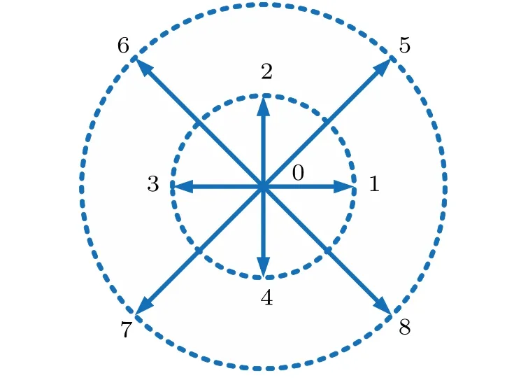
Fig.1.Sketch of the discrete velocity model.

At this point, we have proposed a discrete Boltzmann model that can not only recover the Euler equations, but also capture some TNE effects.After the construction of the physical model,the next step is the numerical design of appropriate discretization schemes.In this work,the second-order Runge–Kutta scheme is chosen for the time derivative in Eq.(1),and the nonoscillatory nonfree dissipative scheme that is at the level of the second-order accuracy is adopted for the spatial derivative.[33]Furthermore, we construct a discrete velocity model,D2V9,in the following mathematical form:

where(0,0)stands for the resting velocity,and the tunable parametersvaandvbare used to control the values of non-zero discrete velocities.Figure 1 depicts the sketch of the discrete velocities,which include a motionless velocity,four velocities with magnitudevain horizontal or vertical directions,and four velocities with sizevbin diagonal directions.Meanwhile,the variableηiis introduced as follows:

农产品科技含量较低，品牌潜力有待挖掘。农业品牌建设必须有过硬的质量和足够的资金作为基础，而过硬的质量又需要由强大的科技作为后盾。为确保品牌农产品的高质量和高效益，农业企业应当加强对农产品的深加工。然而，现阶段卧龙区已认证的无公害品牌除了青华镇永兴农贸公司粗加工玉米面和玉米糁外，其他企业都没有对其产品内在价值进行加工，最终严重影响了企业效益。

Figure 2 delineates the amplitude of vertical velocityuyversus the value of accelerationayat a time instantt=0.01 in the free-falling process.The squares represent the simulation results,and the solid line denotes the exact solutionuy=ayt.Evidently, the DBM results are in excellent agreement with the exact solutions,hence it is confirmed that the matrix inversion method is accurate to calculate the external force on the right-hand of the discrete Boltzmann equation.

3.Simulation and verification

In this section, let us carry out numerical simulations to test the DBM with the proposed discrete velocity scheme.To this end, we consider five typical benchmarks, i.e., the freefalling process, Sod’s shock tube, sound wave, compressible RT instability,and translational motion of a 2D fluid system.

3.1.The free-falling process

First of all,the free-falling process of a physical system is adopted to verify the effectiveness of the force term.The system is homogeneous in a gravity field.Initially,the density isρ=1.0,the flow velocityu=0,and the temperatureT=1.0.Due to the external force,it falls with accelerationayin theydirection as time goes on.The specific heat ratio isγ=1.4,the relaxation timeτ=4×10-6,the temporal step ∆t=10-6,the spatial step ∆x=∆y=10-5, the mesh gridNx×Ny=1×1,and parameters(va,vb,ηa,ηb,ηc)=(1.2,2.0,0.9,3.0,1.3).In addition,the periodic boundary condition is imposed on each boundary.

whereηa,ηb,andηcare adjustable parameters.

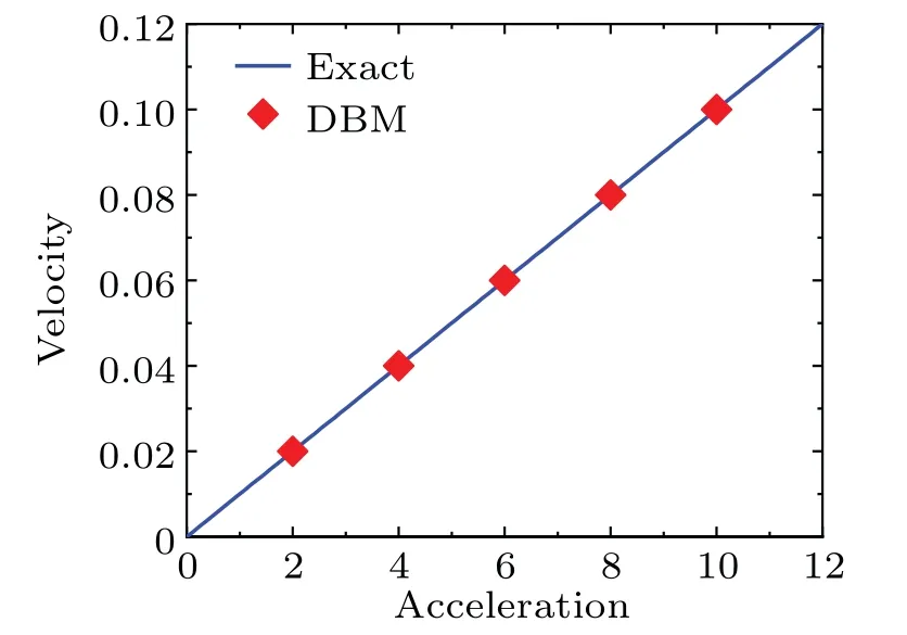
Fig.2.Velocity versus acceleration in the free failing process.

3.2.Sod’s shock tube

The physical reasons for the above phenomena are as follows.In the simplified DBM with D2V9,there are only 9 independent kinetic moment relations satisfied by the discrete equilibrium distribution function.On the contrary, for the DBM with D2V16, there are another 7 kinetic moment relations apart from those in the DBM with D2V9.That is to say,there are 16 independent moment relations satisfied byfeqiin the model of D2V16.The former DBM with D2V9 can recover the Euler equations in the continuum limit and capture a few TNE effects, while the latter model with D2V16 could recover the NS equations in the hydrodynamic limit and offer more TNE information at a higher level of physical accuracy.Consequently,although both DBMs can provide quantities that are qualitatively correct,the model of D2V9 may involve larger errors than the one of D2V16.In fact,to achieve more accurate simulations in situations with various significant TNE effects,we can resort to a DBM where a larger number of moment relationships are required.[29,34]

Figure 5 displays the position of the sound wave travelling forwards in the evolution.The squares stand for simulation results of our DBM, and the solid lines indicate the theoretical solutions ofx=x0+vst.Figure 5(a) shows results in three cases with different specific heat ratiosγand a constant temperatureT=2.0.Figure 5(b)gives cases of various temperatures and a fixed specific heat ratioγ=2.0.Obviously,the numerical results agree well with the exact solutions.Therefore,the model is suitable for fluid systems with various temperatures and specific heat ratios.

Furthermore, let us test whether our DBM has the capability of describing TNE effects.Figure 4 depicts the nonequilibrium quantity∆2,xxin the Sod’s shock tube at timet=0.03.Subplot (a) illustrates the entire computational region, while subplots(b)and(c)show the areas around the rarefaction wave and shock wave, respectively.In each subplot, the results of D2V9,D2V16,[24]and theoretical solutions[26]are compared with each other.Firstly, it can be observed in Fig.4(a) that the simulation results of both D2V9 and D2V16 agree with the analytical solutions on the whole.Secondly,the amplified domain in Fig.4(b) shows that the D2V16 offers simulation results much closer to the theoretical solutions than D2V9.Thirdly, the amplified realm in Fig.4(c) displays slight differences between all numerical and theoretical results.

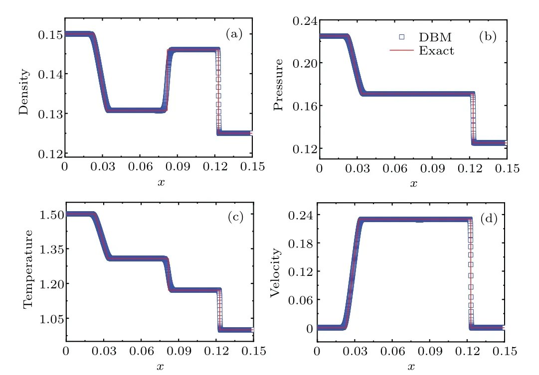
Fig.3.Physical quantities in the Sod’s shock tube: (a)density,(b)pressure,(c) temperature, and (d) horizontal velocity.The solid lines represent the Riemann solutions,and the squares stand for the DBM results.

Figure 3 plots profiles of the density (a), pressure (b),temperature(c),and horizontal velocity(d)in the Sod’s shock tube at the momentt=0.02.Clearly,the leftmost is a rarefaction wave,the middle is a material interface,and the rightmost is a shock wave.The pressure and velocity keep constant while the density and temperature change across the material interface.All physical fields show remarkable gradients around the rarefaction or shock wave,and change sharply near the shock front.It can be found that the DBM results coincide with Riemann solutions on the whole.This indicates that the present DBM can be applied to compressible fluids.

Next,the Sod’s shock tube is simulated to verify that the DBM can be applied to compressible fluids.The initial configuration is

采用英威达行业领先的技术建设PTA装置，是PTA行业对英威达多方面技术和建设工期方面优势的进一步认可。自2012年起，由英威达授权许可的PTA技术总产能达到2100万t/a，约占在中国技术许可的PTA总产能的三分之二。而在这2100万t/a英威达授权许可的PTA产能中，70%的产能基于英威达行业领先的PTA P8技术，该技术为国内新老客户带来了长期的价值。

3.3.Sound wave

In this part,the propagation of a sound wave is simulated in a physical system with the densityρ0=1.0 and velocityu0=0.The relaxation time, temporal step, spatial step, and grid mesh areτ=×10-4, ∆t=10-4, ∆x=∆y=10-3, andNx×Ny=2000×1, respectively.Exerting a small perturbation at the initial positionx0=0.2 will result in the emergence of sound waves that propagate forwards and backwards, respectively.Additionally, the outflow boundary condition and periodic boundary condition are employed in thexandydirections,respectively.

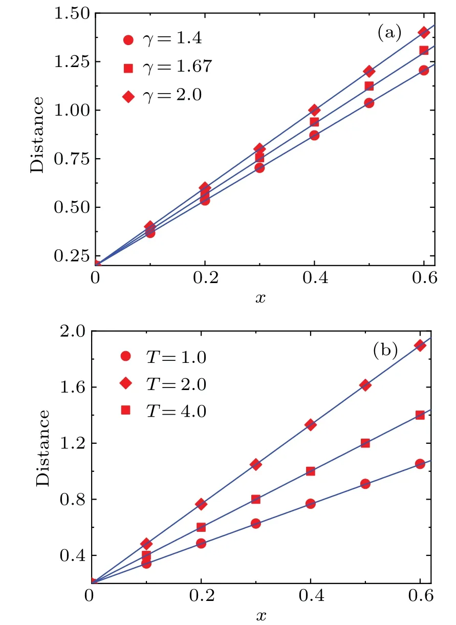
Fig.5.Propagation of the sound wave with various specific heat ratios(a)and various temperatures(b).

where the subscript L denotes the left side 0≤x<0.075 and R represents the right side 0.075≤x ≤0.15.In this simulation, the specific heat ratio isγ=2.0, the relaxation timeτ=10-5, the temporal step ∆t=2×10-6, the spatial step∆x=∆y=5×10-5, and the discrete parametersva=-3.5,vb=1.2,ηa=4.0,ηb=0, andηc=0.In addition, the periodic boundary condition is employed for the top and bottom boundaries, and the inflow and outflow boundary conditions are selected in the left and right boundaries,respectively.

3.4.The compressible RT instability

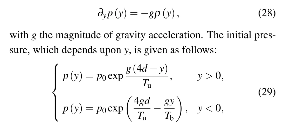
To further verify whether the DBM can effectively simulate complex fluids subjected to external force,we consider the compressible RT instability in a gravitational field.The computational domain,[0,d]×[-4d, 4d],is filled with two layers of fluids with different densities.Between the two media lies the material interface initially located atyc(x)=y0cos(kx),wherek=2π/λ,y0=0.2d, andλ=2drepresent the wave number,the amplitude,and the wavelength,respectively.Initially,the whole system is in hydrostatic equilibrium,wherep0is the initial pressure at the top of the fluid system,andTu(Tb)denotes the initial temperature at the top(bottom).To smooth the transition between the interfaces,a layer is arranged between the two fluids with thicknessW=0.03d,and the initial temperature field is set as where tanh denotes a hyperbolic tangent function.Then, the density field is obtained from the relationρ=p/T.For the simulation, parameters arep0=3.53,τ=1×10-5,ax=0,ay=-g=-1.0,Tu= 1.0, andTb= 2.0, ∆t= 5×10-6,∆x=∆y=1.25×10-4, andNx×Ny=250×2000.Moreover,the symmetric boundary condition is applied in thexandydirections.

The rest of the paper is organized as follows.In Section 2,we introduce the DBM with the proposed discrete velocity model D2V9,utilize the matrix inversion method to calculate the equilibrium distribution function and force term,and show that the DBM could recover the Euler equations in the continuum limit and describe a few TNE effects beyond.In Section 3, the DBM is verified numerically through the benchmarks of the free-falling process, Sod’s shock tube, sound wave,compressible RT instability,and translational motion of a 2D fluid system.Section 4 concludes the paper.

Fig.6.Density contours in the evolution of RT instability simulated by the DBM with D2V9 (in the left four snapshots) and the model of D2V16(in the right four snapshots).[24]

3.5.Translational motion

In this subsection,the movement of 2D fluid without considering external force is simulated to prove that the current model D2V9(1,4,4)has better spatial symmetry and numerical robustness than the previous model D2V9(3,3,3)[27]and possesses higher computational efficiency than D2V16.[24]Here the model(3,3,3)includes three sets of discrete velocities with three directions in each set,[27]and D2V16 contains fours groups of discrete velocities with four directions in each group.[24]

The computation area is a square in size [0,d]×[0,d],where a portion of fluid is placed around the center(d/2,d/2)with a radiusR=d/4.The inner and outer densities areρi=1.1 andρo=1.0, respectively, and there is a transition layer between the two parts.Mathematically,the density is set as follows:

whereW=d/50 is the thickness of the transition layer.The pressure is homogeneous in the system withp=1.0.Meanwhile,two types of flow are under consideration.One is moving rightwards, and the other is flowing in the diagonal direction.The initial configurations of the two cases are plotted in Figs.7(a) and 7(b), respectively.Moreover, the periodic boundary condition is adopted, and simulation parameters ared=0.02,τ=4.0×10-6,∆t=2.0×10-6,∆x=∆y=1.0×10-4,andNx×Ny=200×200.

根据已有研究，在现浇混凝土中添加HEA-JL型抗裂防水可以保证接触界面的黏结强度，提高接触界面的拉拔、劈裂以及抗折强度，减小混凝土的收缩变形，而且可以使局部现浇段有很好的防水能力.选用聚丙烯纤维硅灰水泥浆的界面剂[12]，可以使现浇混凝土与预制混凝土之间紧密结合，二者形成良好的黏结强度，减少混凝土裂缝，将裂缝细化[13].

Hussain等[20]研究发现S.subserrata中化合物53、64、122、142对革兰阳性菌巨大芽胞杆菌和革兰阴性杆菌大肠杆菌具有良好的抑菌作用，对真菌花药黑粉菌的作用较弱。韩立芹[6]报道了旱柳叶的不同提取物的抑菌活性，实验结果显示石油醚层提取物对大肠杆菌、鼠伤寒沙门氏菌具有抑菌作用，最小抑菌浓度为5 mg/mL，醋酸乙酯层提取物对大肠杆菌具有抑菌作用，最小抑菌浓度为25 mg/mL。

Fig.7.The initial configurations of translational motion: horizontal flow(left)and diagonal flow(light).

Fig.8.The horizontal motion of fluid simulated by the models of D2V9 (1, 4, 4), D2V9 (3, 3, 3),[27] and D2V16,[24] in the three rows from top to bottom.The time instants are t=0.01,0.02,0.03,and 0.04 in the four columns from left to right.

Fig.9.The diagonal motion of fluid simulated by the models of D2V9(1,4,4),D2V9(3,3,3),[27] and D2V16,[24] in the three rows from top to bottom.The time instants are t=0.01,0.02,0.03,and 0.04 in the four columns from left to right.

Figure 8 displays the snapshots of a horizontal flow system at four time instantst=0.01, 0.02, 0.03, and 0.04 from left to right.The three rows of simulation results are given by using the models of D2V9 (1, 4, 4), D2V9 (3, 3, 3),[27]and D2V16,[24]respectively.In each subplot, the density reduces from red to blue,and the flow direction is marked with arrows.The dashed black circle in the last column is located at the initial position of the interface between the two media.Given an initial horizontal velocityux=0.5 for the fluids, then it can be predicted that the system moves a distanced=0.02 after a period of timet=0.04,according to the relationshipux=d/tin theory.

It can be seen in Fig.8 that the trajectories of the center of the fluid system provided by the three models are identical.The simulated material interface is symmetric about the centerline in thexdirection and is close to the theoretical position on the dashed black curve.However,upon closer observation of subgraphs in the last column,slight differences can be found among the three simulation results at timet=0.04.(i)In the first row, the dividing interface has little change in thickness,and its shape keeps quite close to a circle.(ii) In the second row, the contact area is wider in thexdirection than in theydirection,and the shape seems an ellipse.(iii)In the last row,the material interface becomes wide gradually due to diffusion and its shape shows perfect symmetry.

In addition, we simulate the motion of a fluid system along the diagonal direction in Fig.9.The components of flow velocity areux=uy=0.5, and the other conditions are the same as those in Fig.8.It can be observed in Fig.9 that the trajectory of the center follows the diagonal direction in both the first and last rows,while the center point departs farther and farther from the diagonal line over time.At the time instantt=0.04,we can observe remarkable differences in the calculated results of the three models: (i)In the first row, the fluid moves in the diagonal direction,the material interface has little change in width, and its shape keeps close to a circle at the predetermined place.(ii)In the second row, the direction of flow velocity completely deviates from the predetermined direction,the contact area becomes wider in the horizontal direction than in the vertical direction, its location deviates far from the exact place,and its shape seems elliptical.(iii)In the last row,the fluid moves along a predetermined trajectory,the dividing boundary becomes thick,both the location and shape are correct.

From Figs.8 and 9, it can be concluded that the models D2V9(1,4,4)and D2V16 have higher physical accuracy and spatial symmetry than D2V9 (3, 3, 3).Moreover, it is worth noting that D2V9 of either (1, 4, 4) or (3, 3, 3) has a higher computational efficiency than D2V16.Table 1 shows the spatial symmetry and computational time of various discrete velocity models in simulations of the diagonal motion.The computation runs on a personal computer with the Intel(R) Core(TM) i7-8550U CPU @1.80 GHz.The computing time required by D2V9 (1, 4, 4) is close to that of the model (3, 3, 3), and is shorter than the one of D2V16.The computation time of D2V16 is about twice as much as that of D2V9.Therefore,the current model D2V9 has a higher computational efficiency.

警察和协警很快就到了。左小龙坐在摩托车上，泥巴不知所措看着。警察到了左小龙跟前，问：“是不是你抢他CD机？”

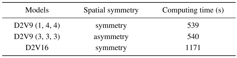
Table 1.Spatial symmetry and computational efficiency of various discrete velocity models.

4.Conclusion

In this work,a DBM with symmetric velocity discretization is presented for compressible flow system that is subjected to external force and possesses an adjustable specific heat ratio.We constructed a discrete velocity scheme, D2V9 (1, 4,4),which assumes a resting velocity,a group of velocities with the same magnitudevain four horizontal or vertical directions,and a group with sizevbin four diagonal directions.This discretized velocity model has better spatial symmetry and numerical accuracy than the model in Ref.[27]and owns higher computational efficiency than the one in Ref.[24].In addition, the matrix inversion method is adopted to calculate the discrete equilibrium distribution function and force term,both of which satisfy nine independent kinetic moment relations.Moreover, the DBM could be used to study a few thermodynamic nonequilibrium effects beyond the Euler equations that can be recovered from the kinetic model in the hydrodynamic limit via the Chapman–Enskog expansion.Finally,the method is verified through typical numerical simulations,including the free-falling process,Sod’s shock tube,sound wave,compressible RT instability,and translational motion of a 2D fluid system.These simulations show that the current DBM can effectively investigate compressible flows with or without external force and could provide some nonequilibrium information.

财务内控管理应该是全面的，全面的企业财务内控管理机制应该全面覆盖事前控制、事中控制以及事后控制这些环节。

Acknowledgements

Project supported by the National Natural Science Foundation of China (Grant Nos.51806116, U2242214, and 11875329), Guangdong Basic and Applied Basic Research Foundation (Grant No.2022A1515012116), and the Natural Science Foundation of Fujian Province, China (Grant Nos.2021J01652 and 2021J01655).