Adaptive Graph Convolutional Recurrent Neural Networks for System-Level Mobile Traffic Forecasting
2023-11-06YiZhangMinZhangYihanGuiYuWangHongZhuWenbinChenDanshiWang
Yi Zhang ,Min Zhang ,Yihan Gui ,Yu Wang ,Hong Zhu ,Wenbin Chen ,Danshi Wang,*
1 Beijing University of Posts and Telecommunications,Beijing 100876,China
2 The Intelligent Network Innovation Center of Chinaunicom,Beijing 100048,China
*The corresponding author,email: danshi_wang@bupt.edu.cn
Abstract: Accurate traffic pattern prediction in largescale networks is of great importance for intelligent system management and automatic resource allocation.System-level mobile traffic forecasting has significant challenges due to the tremendous temporal and spatial dynamics introduced by diverse Internet user behaviors and frequent traffic migration.Spatialtemporal graph modeling is an efficient approach for analyzing the spatial relations and temporal trends of mobile traffic in a large system.Previous research may not reflect the optimal dependency by ignoring inter-base station dependency or pre-determining the explicit geological distance as the interrelationship of base stations.To overcome the limitations of graph structure,this study proposes an adaptive graph convolutional network (AGCN) that captures the latent spatial dependency by developing self-adaptive dependency matrices and acquires temporal dependency using recurrent neural networks.Evaluated on two mobile network datasets,the experimental results demonstrate that this method outperforms other baselines and reduces the mean absolute error by 3.7 % and 5.6 %compared to time-series based approaches.
Keywords: adaptive graph convolutional network;mobile traffic prediction;spatial-temporal dependence
I.INTRODUCTION
According to Cisco’s latest statistical survey,8.4 billion handheld or personal mobile-ready devices will be connected to the Internet by 2022,and the mobile traffic volume will increase at an annual growth rate of 46 percent from 2017 to 2022[1].In the incoming 5G era [2],the real-time and delay-sensitive traffic from various applications(such as autonomous vehicles and virtual reality) poses major challenges to mobile networks.
If future traffic volume can be estimated using historical data,a corresponding resource adjustment can be made in advance to improve resource utilization,and avoid network congestion [3,4].Time seriesbased analysis and prediction have recently been successfully studied [5–11].Statistical and deep learning models are two prominent examples of data-driven methods.In the statistics field,autoregressive integrated moving average (ARIMA) [12] is the general class of models for forecasting a stationary time series.Additionally,deep learning approaches that effectively learn the relations on the time axis have been widely applied to various traffic tasks,including multilayer perceptron (MLP),one-dimensional convolutional neural networks (CNNs),and recurrent neural networks(RNNs),and WaveNet.
Previous researchers have reported that diverse Internet user behaviors and frequent user mobility introduce tremendous temporal and spatial dynamics to data traffic [8].Therefore,interactions and behavior patterns [13] among base stations need to be considered in traffic prediction for multiple base stations.To address this issue,researchers have attempted to introduce spatial features in new models.By converting network-wide traffic volume into a series of static 2D images,and utilizing a 3-dimensional convolutional neural network (3D-CNN) [9] or convolutional long short-term memory (ConvLSTM) [14] to simultaneously capture spatiotemporal relations.However,converting global traffic to images is a crude method,and its performance may suffer from the problem of sparse matrices.
The newly proposed graph convolutional network(GCN) provides a solution that can extract the spatial dependency between base stations from non-Euclidean data [15].Then by combining with RNNs[16,17]or CNNs[18],the GCN can take full advantage of both spatial and temporal features.However,there are still several bottlenecks in the current GCN that need to be resolved [19].The GCN model assumes that the graph topology of the dataset reflects the authentic node correlations without verification and the topology is incapable of learning new connections.There are some circumstances when an interdependent relationship exists between two nodes but a connection is missing.For example,if two base stations in different downtown areas,where the majority of populations consists of office workers,are far apart,the similarities of base station traffic patterns may not be reflected in the graph topology.
In this study,the goal is to forecast mobile traffic on a set of practical base stations where the historical traffic volume and location are known,as illustrated in Figure 1.The critical assumption is that a base station’s future traffic is affected by its own and other base stations’historical information.
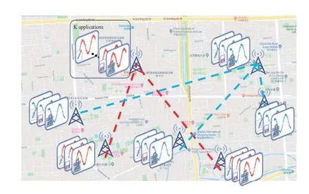
Figure 1.Geographical location of nodes marked on a map. Each base station has dynamic traffic features including video-streaming,web-browsing,file transfer,etc. The dashed lines denote proximity between base stations.
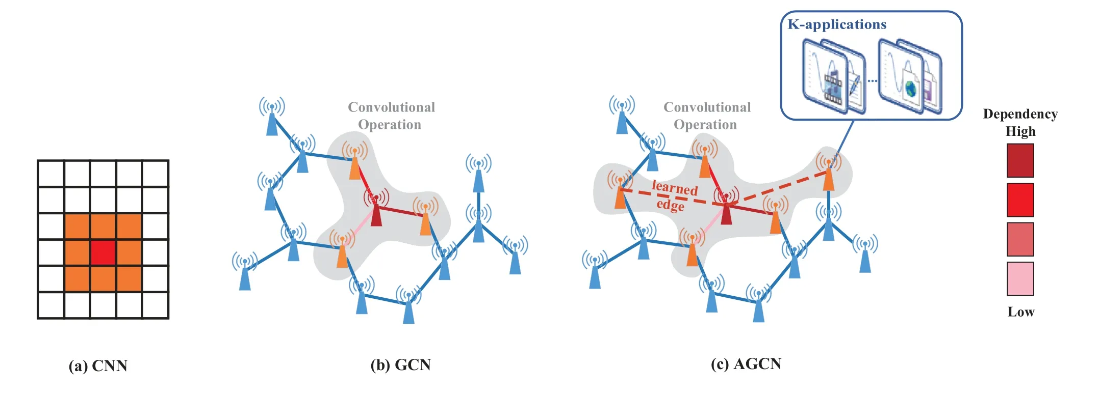
Figure 2.Convolution operation comparison. Red point: center of the kernel. Orange points: coverage of the kernel.(a) classical CNN on an image;(b) GCN,spatial-based convolutional operation on a graph;(c) AGCN,operation on an adaptive graph. Learned edges are red dash lines. The color of an edge indicates the dependency weights between nodes.
To address these issues,a GCN-based model called as the adaptive graph convolutional network(AGCN)is proposed.In this model,the graph topology structure is no longer fixed,but is optimized through endto-end training.The proposed AGCN consists of an RNNs or WaveNet framework and leverages a selfadaptive graphical representation to learn inter-base station dependency.RNNs or WaveNet captures traffic trends through time steps.The proposed model consistently outperformed traffic forecasting baselines when evaluated on two real-world traffic datasets.
The pair-wise spatial correlations between base stations are represented using a directed graph where the nodes are traffic volume and the edge weights denote proximity of the base station pairs.The AGCN model can capture the latent spatial relations of nodes in an end-to-end manner.
Experimental results on the Guangzhou and Hangzhou traffic network datasets demonstrate that the mean absolute percentage error(MAPE)and mean absolute error (MAE) of the proposed AGCN model are reduced by more than 5.6 % and 3.7 %,respectively,compared to time-series based models.
II.METHODOLOGY
In this section,a mathematical description of the prediction task and illustration of architecture of the proposed framework is provided.
2.1 Task Definition
In this task,the graph is represented byG=(V,E),whereVis the set of base station nodes,and E is the set of edges in a graph.The graph adjacency matrix is denoted asA∈RN×N,whereNis the size ofV.At each time stept,the graphGhas a feature matrixXt∈RN×KwhereKrepresents the number of mobile traffic features.Given a graphGand historicalSstep signalX(t-S-1):t,the task is to learn a function that can predict the nextTtime steps signalXt+1:(t+T).The inputs and outputs of function are presented below.The inputsX∈RS×N×Kand outputsX∈RT×N×Kare three-dimensional tensors.SandTare the lengths of the historical and prediction time series,respectively.
2.2 Graph Convolution Layer
Graph convolution network can model the dynamicity of mobile traffic as an information dissemination process and efficiently capture a node’s spatial feature given its adjacency matrix.From a spatial perspective,graph convolution network utilizes the weighted average value of the features of a node and its neighbors.The first approximate convolution on the graph is defined as[15]:
2.3 Adaptive Graph Convolution Layer
In a previous study,Li et al.proposed a self-adaptive adjacency matrix that,independently learned the hidden spatial dependency,and proved to be powerful in spatial-temporal modeling[19].In this paper,we use a parameter matrixMkto parameterize the distance matrixDk(xi,xj),so that the graph itself becomes trainable.Meanwhile,the graph topological structures of samples are updated to minimize training losses.In AGCN,for each featurek∈K,an adaptive adjacency matrixis used to model the spatial dependency,respectively.
whereDk(xi,xj) is Mahalanobis distance between base stationxiandxjand adjacency matrixis constructed by distance matrix with a Gaussian kernel [20].The positive semidefinite matrixMkis a parameter matrix.IfMk=I,Eq.(3) reduces to the Euclidean distance.In this model,each adaptive adjacency matrixcan model the spatial dependency of one traffic feature and minimize the predictive losses during training.
Given graphGand its adjacency matrixAand degree matrix,the normalized graph Laplacian matrixLis obtained by:
Ldetermines both the node-wise connectivity and the degree of vertices.Laplacian is a symmetric positive definite matrix and its eigendecomposition gives a set of eigenvectorsUformed by.UseUas graph Fourier basis and Λ as the spectral representation of graph topology,graph Laplacian is diagonalized asL=UΛUTTo model the spatial feature,we use a spectral filtergθ(Λ)that parameterizes the graph Laplacian.Given LaplacianL,featuresXand parameters Γ,the functionF(L,X,Γ)outputs the spectrum of Laplacian.Finally,the AGCN layer is primarily formulated as:
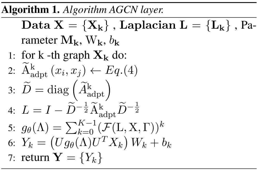
Atk-th layer the transform matrixWk∈Rn×nand the biasbk∈Rn×1are trained along with metrics Mk,where n is the input graph size.A the AGCN layer,we have the parameters M,W,b of O(k×n2)learning complexity.Compared with GCN,the adaptive graph convolution kernel construct and learn unique residual Laplacian matrix{Lk}for individual feature.
2.4 Temporal Dependency Modeling
Gated recurrent unit (GRU) models and long shortterm memory (LSTM) are prominent and powerful variants of RNNs,and are particularly effective for time series prediction problems [6].In addition,WaveNet is also a classic convolutional network model for time series processing.Therefore,GRU,LSTM,and WaveNet were adopted as the temporal dependency model to capture temporal trends of nodes in this study.
In multi-step ahead forecasting,the sequence to sequence architecture is employed.The encoders and decoders are GRU or LSTM cells.The historical time series is fed into the encoder and its final states are used to initialize the decoder.The decoder generates predictions based on the previous time-step prediction.The same multi-step prediction can be performed in the WaveNet model,as shown in Figure 3.
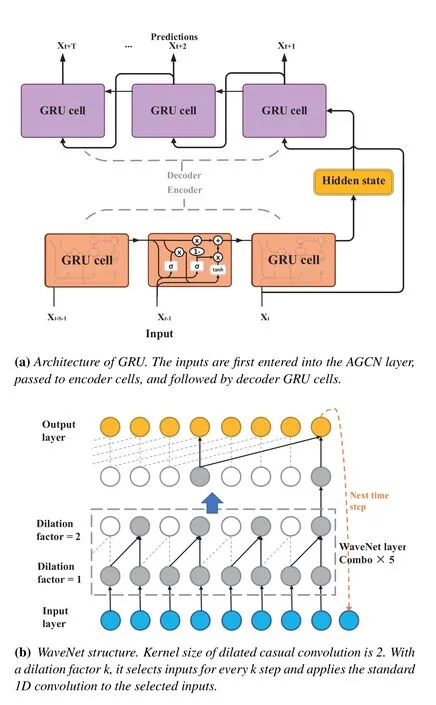
Figure 3.Architectures of GRU and WaveNet.
2.5 Framework of AGCN-Based Architecture
A framework for an adaptive graph convolution network with a temporal neural network model is proposed for both spatial and temporal dependency modeling,using GRU as an example,as shown in Figure 4.By stacking the spatial and temporal layers,the proposed model is able to capture the spatiotemporal dependencies among time series and be applied to time series prediction tasks.A DNN layer with a ReLU activation function is the output layer of the model.The entire model is trained by maximizing the likelihood of generating the target future time series through backpropagation over time.
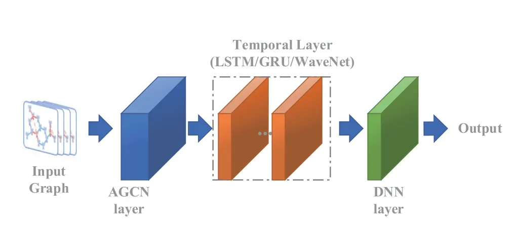
Figure 4.AGCN network configuration. Directly feed it on the original graph-structured data and their initial graphs.
III.EXPERIMENTS AND RESULTS
3.1 Datasets and Preprocessing
The proposed model is evaluated on two real-world mobile traffic datasets from practical network of a telecom operator,consisting of 46 days of mobile traffic from 100 base stations in Hangzhou city and oneweek mobile traffic of 12 base stations in Guangzhou city.Datasets contain fourteen attributes,i.e.,video,web,VoIP,social networks,within which every item is time series.Details of two datasets are depicted in Table 1.This paper aims to explore the pattern capture capability of neural network models for time series data.Therefore,we used traffic data and base station geographic information and no external features were used.
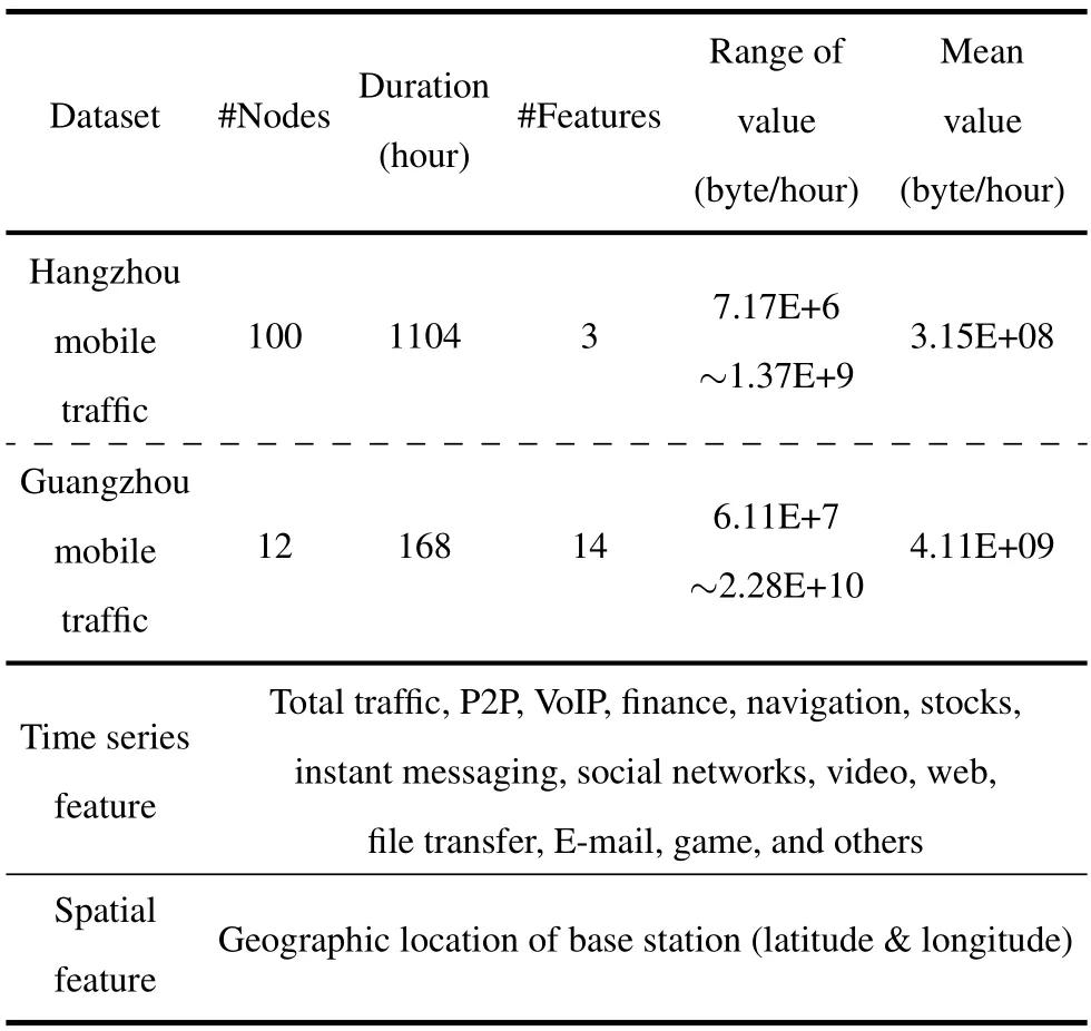
Table 1.Datasets descriptions and all features.
According to two datasets,the traffic volume can peak at 22.8GB per hour during congestion hours,which is three orders of magnitude greater than offpeak hours for the same base station.This shows that mobile traffic values change more drastically and have a wider dynamic range than other time series,such as road traffic data[5,16].
In the preprocessing stage,the traffic of each node is aggregated into a one-hour window.The dataset is split in order of time with the first 80 % for training and the last 20%for testing.All tests use 48 h(S=48)as the historical time window to forecast traffic conditions in the next 1,2,and 4 hours.In order to obtain a more normal intra-series values distribution,raw traffic values were transformed by natural logarithm and Zscore normalization,as defined in Eq.(6).Each base station traffic was normalized independently.
where mean(·)and std(·) are arithmetic mean and standard deviation,respectively.
3.2 Baseline Models
The AGCN-based model was compared with the following deep neural networks(NNs).
(1) ARIMA: autoregressive integrated moving average is a linear model,commonly used in predicting future points in the series.The autoregressive terms p is 4,the number of differences needed for stationarity d is 2,and the lagged forecast errors in the prediction equation q is 1 (2) WaveNet: Diffusion convolution network architecture for sequence generation.We use 10-layers WaveNet with a sequence of dilation factors=(1,2,1,2,1,2,1,2,1,2),kernel size=2,and the number of output filters=24.Dropout with p=0.3 is applied to the outputs of the WaveNet convolution layer.Convolution kernel weights matrix is initialized by Glorot uniforminitializer.(3)LSTM:One-layer unidirectional LSTM with 64 memory cells [6].L1 and L2 regularization is used,where L1=0.01 and L2=0.004.(4)GRU:an RNN variation model that exhibits better performance on smaller datasets and is set to one unidirectional layer with 64 memory cells.(5)GCNbased models integrate a graph convolution layer anda time series layer.We tested three GCN-based models,including GCNWaveNet,GCN-LSTM,and GCNGRU [16].For graph convolution kernel,the initial adjacency matrix of the nodes is constructed by the geographical distance between the base stations.For comparison reasons,the parameters of temporal layer in the GCN-based model are consistent with those in pure temporal models.(6) AGCN-based models are set to the same hyperparameters as GCN-based models.
3.3 Experimental Setups
Our experiments are conducted under a cloud computational environment with two core 2GHz CPU,16GB memory and one NVIDIA Tesla P100 GPU card.All models in this study were implemented on the TensorFlow platform.For all NNs,the Adam optimizer was used with the initial learning rate of 0.001,and the decay parameter was set to 0.95.A grid search was adopted to tune other hyperparameters by measuring performance on validation data.We used early stopping to monitor the performance of the model for every epoch on a held-out validation set during the training,and terminate the training conditional on the validation performance.
Experiments were conducted with two configurations to verify the effectiveness of the proposed adaptive adjacency matrix.(1) GCN: Original version of the GCN defined in Eq.(2).The adjacency matrix is set by the geographic graph structure.(2)AGCN:Proposed adaptive graph convolution layer as defined in Eq.(3).
The evaluation metrics include the MAPE,MAE,and coefficient of determination (R2).MAPE was chosen as the training target function in these experiments,which is computed by:
whereXandare the ground truth traffic and the model predictions,respectively.
3.4 Experimental Results
The comparative performances of AGCN-based and other baseline models’predictions for 1,2,and 4 hours ahead of the mobile traffic datasets are summarized in Table 2.The results were evaluated by averaging twenty runs.It was found that spatial-temporal GCN models achieved little improvement than temporalonly models.The AGCN approaches surpassed previous non-adaptive GCN approaches due to the extracted latent spatial information,thus achieving the optimal performance in all evaluation metrics.The method outperformed others in predicting extremely light or heavy traffic and has the potential to be applied to traffic volumes spanning a wide dynamic range.
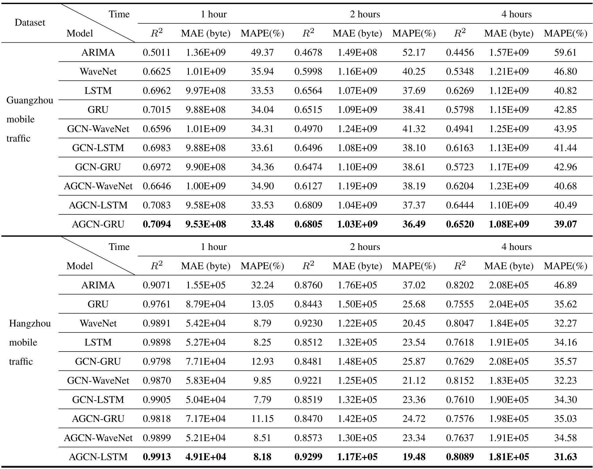
Table 2.Performance comparions of AGCNs and baseline models.
To further investigate the performance of AGCNbased models,boxplots and the training curves of test loss are shown in Figures 5 and 6.Figure 5 indicates that the AGCN-based structure has better performance for all RNNs and the WaveNet model.Figure 6 also indicates that the AGCN-based models can achieve much faster training procedures and easier convergences.
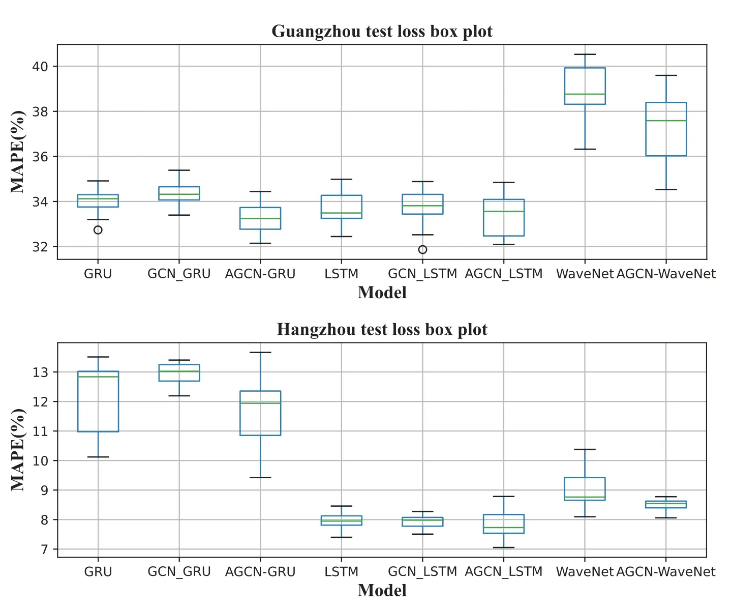
Figure 5.Box plot of one-hour prediction MAPE.
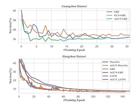
Figure 6.Learning curve of one-hour prediction: test loss versus training epochs number.
As illustrated in Figure 7,AGCN-GRU captures the trends more accurately and generates more stable predictions than the other models.In particular,there is a sharp green spike produced by GCN-GRU,which deviates far from real values,and a large degree of hysteresis upon green curves was observed.On the contrary,the curve of AGCN-GRU is more conservative and goes in the middle of real values all the time.This shows that the AGCN-based models work better than with the non-adaptive GCN models.
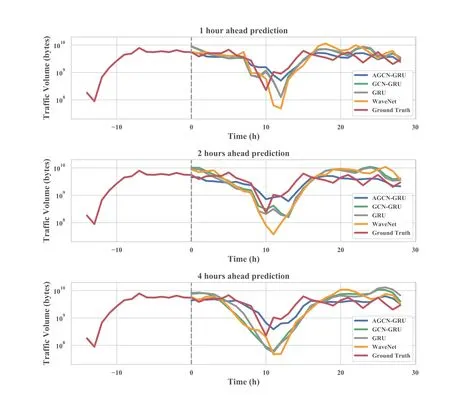
Figure 7.Visualization of 1,2,and 4-hour total traffic forecasting results in Guangzhou dataset.
To provide an additional perspective on the value of employing these proposals for mobile traffic forecasting,a heatmap of predicted and true traffic across the entire network on a randomly selected day (Jan.12,2018)is displayed in Figure 8.The similarity between the shapes in the two heat maps shows that the proposed model is capable of fitting true spatial-temporal patterns.The cumulative distribution function (CDF)of per hour traffic volume in Guangzhou dataset is shown in Figure 9,which can be fitted by the AGCNGRU model prediction distribution.
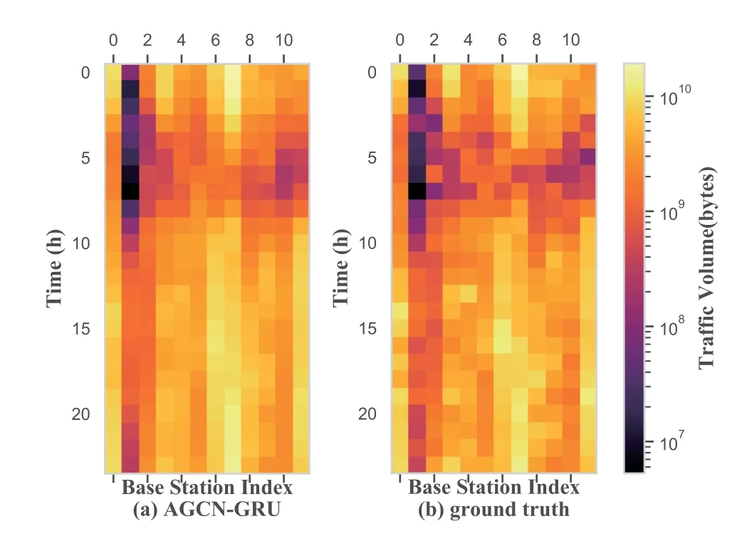
Figure 8.Heatmaps of one-hour ahead traffic forecasting of AGCN-GRU model and ground truth of Guangzhou dataset on 12/01/2018.
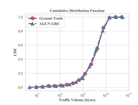
Figure 9.Cumulative distribution function (CDF) of AGCN-GRU model one-hour ahead prediction and ground truth of Guangzhou dataset.
The following observations can be made.(1)For all prediction methods,MAE increases with the forecasting horizon (from 1 to 4h).This is because the temporal dynamic becomes increasingly non-linear with the growth of the horizon.(2)The GCN-based model performs similarly to RNNs.This could be explained by the fact that recurrent neural networks play a vital role in the spatial-temporal prediction model,and the explicit geological graph structure does not reflect the true dependency.Without graph modeling,this network has a similar encoding capacity to RNNs for the time series.(3)Compared to the GCN model,the AGCN-based model reduces the mean absolute error by 3.7 %,6.4 %,and 7.7 % in the 1,2,and 4 hours forecasting horizons,respectively.The AGCN model has superior performances in balancing time consumption and parameter settings,due to the self-adaptive graph structure.
3.5 Effects of Adaptive Adjacency Matrix
Table 2 shows that the adaptive GCN model performs better than the non-adaptive GCN model.The adjacency matrices are initialized using geological distance and learn the adaptive graph topology structure according to the data.Alternatively,AGCN is able to achieve excellent performance after training.This indicates that prior graph knowledge does not reveal the optimal spatial dependency of nodes,and it could be optimized during training.
In Figure 10,the learned self-adaptive adjacency matrix under the configuration of the AGCN model is further investigated.Some blocks have more highvalue points than others,such as column 2 in the orange box.This suggests that the #2 base station is highly influential to other base stations(#0,1,3)in the graph,even if there is a distant geographical relationship.The graph will be updated during training since the network is trained to optimize the distance metric and feature transform for training data.The experiment demonstrated a close correlation between the updated graph and network performance.
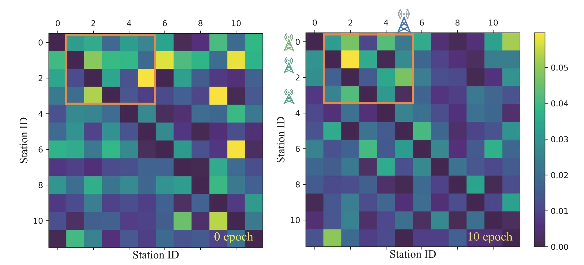
Figure 10.Two heat maps of an example of learned self-adaptive adjacency matrices for the 12 base stations. Left is before training,and the other is after the 10 epochs adjacency matrices. The selected part of the matrix indicates the learning process of the adjacency graph.
3.6 Computation Time
We compare the computation cost of AGCN with other baselines in Figure 11.
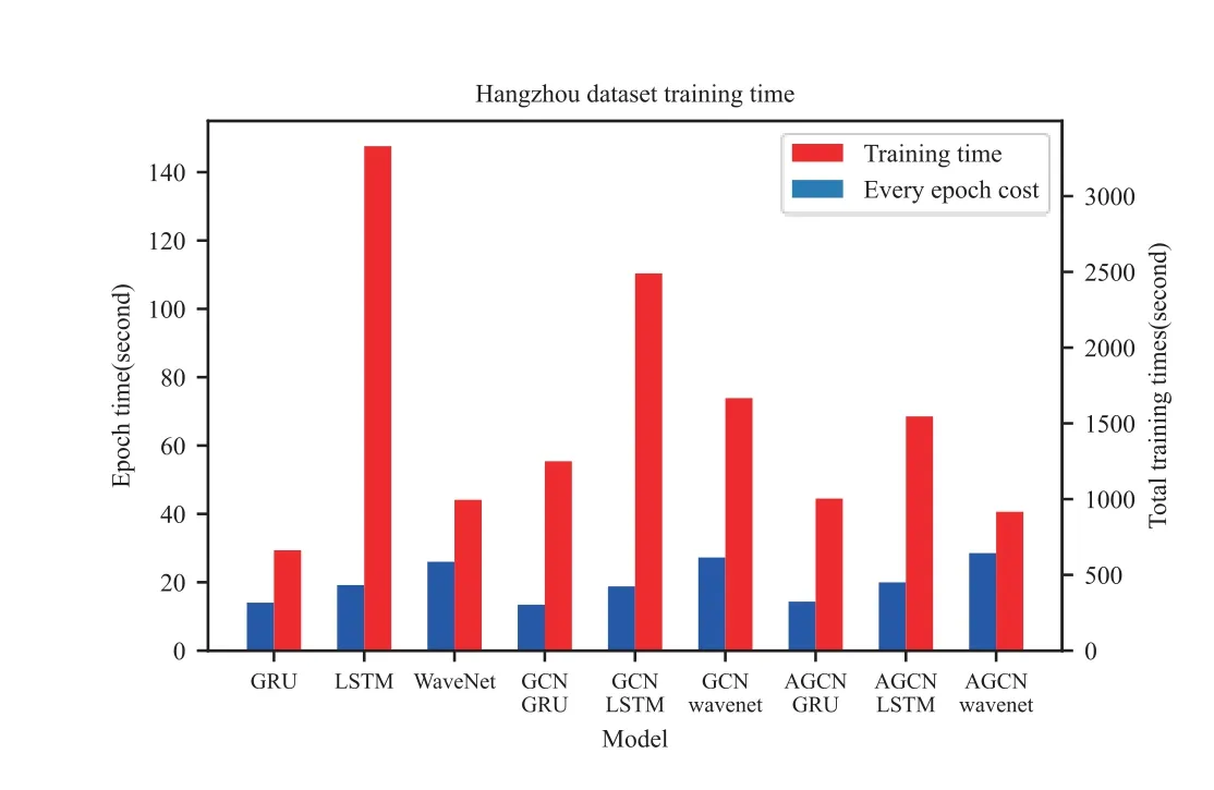
Figure 11.Histogram of training time cost and time per epoch.
WaveNet-based models run slower than RNN models in training.This is because that we use a deeper WaveNet structure than LSTM and GRU.Because GCN and AGCN models have a deeper network structure and a larger number of parameters,the training time cost of every epoch increased.But the model based on AGCN converges faster than the GCN models and pure time series model,so the number of epochs needed to complete the training is less.
IV.CONCLUSION
In this study,the global traffic of a mobile network was formulated as a spatiotemporal graph structure and an adaptive graph convolutional recurrent neural network was proposed to automatically learn latent spatial dependencies from data.A new approach to graph modeling was established,where the latent dependency structure of a system is unknown and needs to be discovered.When evaluated on two real-world traffic datasets,the proposed AGCN-based model achieved comparatively better performance than the other baselines.For future work,this approach will be exploited to benefit advanced technologies such as network slices and traffic scheduling.
ACKNOWLEDGEMENT
This work was supported by the National Natural Science Foundation of China (61975020,62171053).(Corresponding authors: Danshi Wang).
杂志排行
China Communications的其它文章
- Learning-Based Dynamic Connectivity Maintenance for UAV-Assisted D2D Multicast Communication
- AIGC Scenario Analysis and Research on Technology Roadmap of Internet Industry Application
- Dynamic Visible Light Positioning Based on Enhanced Visual Target Tracking
- Ultra Dense Satellite-Enabled 6G Networks: Resource Optimization and Interference Management
- Analysis and Optimization of Validation Procedure in Blockchain-Enhanced Wireless Resource Sharing and Transactions
- Anti-Jamming and Anti-Eavesdropping in A2G Communication System with Jittering UAV
