Identifying Host Galaxies of Extragalactic Radio Emission Structures using Machine Learning

Kangzhi Lou,Sean E.Lake,and Chao-Wei Tsai,3

1 National Astronomical Observatories,Chinese Academy of Sciences,Beijing100101,China;cwtsai@nao.cas.cn,lake@nao.cas.cn

2 University of Chinese Academy of Sciences,Beijing100049,China

3Institute for Frontiers in Astronomy and Astrophysics,Beijing Normal University,Beijing102206,China

Abstract This paper presents an automatic multi-band source cross-identification method based on deep learning to identify the hosts of extragalactic radio emission structures.The aim is to satisfy the increased demand for automatic radio source identification and analysis of large-scale survey data from next-generation radio facilities such as the Square Kilometre Array and the Next Generation Very Large Array.We demonstrate a 97% overall accuracy in distinguishing quasi-stellar objects,galaxies and stars using their optical morphologies plus their corresponding mid-infrared information by training and testing a convolutional neural network on Pan-STARRS imaging and WISE photometry.Compared with an expert-evaluated sample,we show that our approach has 95% accuracy at identifying the hosts of extended radio components.We also find that improving radio core localization,for instance by locating its geodesic center,could further increase the accuracy of locating the hosts of systems with a complex radio structure,such as C-shaped radio galaxies.The framework developed in this work can be used for analyzing data from future large-scale radio surveys.

Key words: techniques: image processing–surveys–methods: data analysis

1.Introduction

Radio galaxies,characterized by their enormous radio emission structures,are a subclass of active galactic nuclei(AGNs) that span up to several Mpc with total radio power exceeding 1039W(Chaisson&McMillan 2014).The extended radio galaxies often display unique radio emission structures,such as jets and lobes reaching outside their host galaxies’optical counterparts.The large morphological diversity of these radio giants is believed to be powered by the supermassive black holes’ accretion in the nuclei of their host galaxies.The non-thermal and polarized radio emissions are dominated by synchrotron radiation of AGN-accelerated relativistic electrons and positrons in the magnetic fields (Hardcastle &Croston 2020).The collimated relativistic particles can reach beyond the host galaxy and,sometimes,collide with the cold interstellar medium,creating extremely luminous hotspots.

Following the methods of Fanaroff &Riley (1974),the morphology of radio galaxies is usually classified by whether they exhibit a brightness profile that decreases from the core or increases.The former are called FR-I sources and the latter are FR-II and they often have bright hotspots at the ends of the lobes.However,this basic classification scheme is no longer sufficient to characterize the complicated morphology of radio galaxies that are discovered with an increasing speed in largescale radio sky surveys.For example,a radio galaxy with two pairs of bent jets or lobes that form a shape resembling the letters C,X or Z is usually referred to as a C-shaped,X-shaped or Z-shaped radio galaxy,respectively.Figure 1 shows a collection of radio galaxies with complex radio emission structures.These complicated morphological features create a big challenge in identifying the optical counterpart of their host galaxies.

Most of the host galaxies of radio galaxies are large elliptical galaxies (Kuźmicz et al.2019).However,some of the doublelobed radio sources with structures on larger than kiloparsec scales are found to be hosted by disk galaxies (e.g.,Ledlow et al.1998,2001;Croston et al.2008;Hota et al.2011;Tsai et al.2013;Mao 2015;Mulcahy et al.2016;Gao et al.2023).There is not,yet,a consensus model that describes the formation processes of these radio structures and the interaction between the radio emission and their host galaxies.Further studies will require a sample of galaxies with different morphologies,evolutionary states,AGN accretion rates and galaxy environments (e.g.,Krause et al.2019).

The radio emission in a radio galaxy system can be extended from a few kpc to Mpc.The projected image of these radio structures can be well separated on the sky from their host galaxies.Thus,identifying the optical host galaxies in the radio galaxy systems is far more challenging than finding the optical counterparts with a simple cross-matching of the coordinates of the radio and optical sources.The traditional method for crossmatching radio galaxies with their optical hosts is by experts’visual inspection (e.g.,Norris et al.2006;Taylor et al.2007;Middelberg et al.2008;Gendre&Wall 2008;Grant et al.2010;Gendre et al.2010;Lin et al.2010).For example,Norris et al.(2006) analyzed 784 radio emission components from a 3.7 deg2field surrounding the Chandra Deep Field-South(CDF-South) in the Australia Telescope Large Area Survey(ATLAS) and cross-matched them with the infrared sources from theSpitzerSWIRE survey.A similar effort was made on the deeper radio data by Middelberg et al.(2008),who grouped 1366 radio components into 1276 sources and matched 1183 of them with infrared sources.For the data from the large-scale radio sky surveys,the host identification can rely on citizen scientist projects (e.g.,Banfield et al.2015).These efforts usually involve thousands of trained citizen scientists in crossmatching a large number (hundreds of thousands or more) of radio sources with their infrared counterparts and conducting visual inspections.However,even citizen scientist projects will find it challenging to analyze the expected millions of radio sources in upcoming radio surveys (Norris 2017).An alternative solution to this enormous data challenge is to use automated algorithms and methods.

The automated host identification approaches are generally of two types: statistics-based cross-matching and machine learning methods.The former often utilize the likelihood ratio technique(Sutherland&Saunders 1992;McAlpine et al.2012;Weston et al.2018;Williams et al.2019;Kondapally et al.2021),while some use Bayesian hypothesis testing (Fan et al.2015,2020).However,these methods cannot be easily used to cross-match between extended radio structures and sources from other bands and they also often involve processes too complex to be practically applied to large surveys.The machine learning approach describes a class of methods that learn approximations of functions for host identification based on existing training samples from the work of experts or citizen scientists to train machine learning models (e.g.,Alger et al.2018).

This paper demonstrates a novel and efficient supervised framework for identifying hosts of radio galaxies by combining multi-band source feature extraction with an image processing technique that uses convolutional neural networks(CNNs).Our joint multi-band CNN models can achieve high accuracy in finding the best optical host candidates.We show that classifying the optical host candidates before carrying out the cross-identification task can boost the accuracy of optical host identification.Our approach is in contrast to typical CNN applications for cross-matching that involve creating a simple machine learning model and manually picking source features for the model to train on.The paper is organized as follows.In Section 2.2 we describe the radio galaxy samples and the multiwavelength data used in this work.In Section 3 we discuss the data processing and the network design of our machine learning framework.We present the results of applying our machine learning model on expert-inspected samples (Norris et al.2006)and analyze the model’s performance in Section 4.In Section 5,we discuss our results and evaluate the possible improvements that can be made to our method.We summarize the whole work in Section 6.

2.Feature Data Sets and Sample Selections

2.1.Feature Data Sets

This work uses radio data of objects in our training and testing samples from the VLA Sky Survey (VLASS;Lacy et al.2020),optical data from the Panoramic Survey Telescope and Rapid Response System (Pan-STARRS;Chambers et al.2016) and mid-infrared data fromWide-field Infrared Survey Explorer(WISE;Wright et al.2010).We used VLASS image cutouts during the process to conduct the morphology analysis of radio galaxies.The Pan-STARRS sky survey provides optical sources for evaluation as host galaxy candidates and the image cutouts containing them.WISE's W1 and W2 magnitudes of the optical sources in the field are also used to better differentiate source types,especially stars and AGNs.

VLASS is an ongoing radio continuum sky survey at 2–4 GHz with an angular resolution of(Gordon et al.2021).The sensitivity has a 1σ goal of 70 μJy beam−1in the three-epoch coadded data and 120 μJy beam−1in the singleepoch images.VLASS’s observations began in September 2017,with the projected observing finish time set in 2024.VLASS is expected to cover the whole sky with δ ≥−40°,a total of 33,885 deg2,with VLA observations from 2017 to 2024.As of the writing of this paper,VLASS has completed its first two epochs.4https://www.cadc-ccda.hia-iha.nrc-cnrc.gc.ca/en/vlass/.Prior to the release of the single-epoch highquality images,“quick look” images with a pixel size of 1″processed using a streamlined version of the CLEAN algorithm(Högbom 1974)were released.All of the radio images used in this research come from the VLASS Quick Look image products in epoch 2,which suffer less from positional errors,flux density errors and ghost artifacts (Gordon et al.2021).5https://archive-new.nrao.edu/vlass/quicklook/.

Pan-STARRS is an optical survey in five bands(grizyP1)that covers the entire sky north of decl.−30°.The first phase of the program (Pan-STARRS1) comprises the 3π Steradian Survey and the Medium Deep Survey.The mean 5σ point source limiting sensitivities in the stacked 3π Steradian Survey ingrizyP1are 23.3,23.2,23.1,22.3 and 21.4 AB magnitudes,respectively.WISEis an infrared sky survey that covers the whole sky at 3.4,4.6,12 and 22 μm (W1,W2,W3 and W4,respectively) with an angular resolution ofandrespectively.The 5σ point source sensitivities are better than 0.08,0.11,1 and 6 mJy in unconfused regions in its four bands,respectively.The resolutions and sensitivities of these surveys are sufficient for us to determine the host galaxies of radio galaxy systems in the local universe.

2.2.Sample Selection

2.2.1.Radio Sample Selection

Identifying the host of a radio galaxy is challenging,especially when the emission region of the target radio galaxy is extended well beyond its optical structures.As a result,there is a significant amount of uncertainty about a host galaxy’s location relative to the corresponding radio galaxy.Much research has been done on cross-matching radio sources and sources from other bands.Visual inspection by experts can handle a small number of radio sources detected in small-scale radio surveys (e.g.,Laing et al.1983;Norris et al.2006;Middelberg et al.2008).Large-scale visual inspection to identify the optical host galaxies of the radio galaxy systems has been done by citizen scientist projects such as the Radio Galaxy Zoo project (RGZ;Banfield et al.2015)).The RGZ alone has provided over 75,000 radio-host cross-identifications in addition to radio source morphology information (Alger et al.2018).

Automatic methods have also been studied to handle crossmatching the increasing number of radio sources with their counterparts in other bands.As discussed in Section 1,the complex yet reliable statistical methods such as the likelihood ratio technique have been successfully shown to produce the probabilities of being the true optical host candidate for all the optical sources in the field.Fan et al.(2015,2020)adopted the Bayesian hypothesis testing method to achieve a similar goal.On the other hand,Alger et al.(2018) adopted machine learning methods in dealing with the cross-matching problem.In that work,the model was trained on expert crossidentifications from Norris et al.(2006) and volunteer crossidentifications from the RGZ project.

Norris et al.(2006) presented the results from the Australia Telescope Large Area Survey (ATLAS),which consists of deep radio observations of a 3.7 deg2field surrounding the Chandra Deep Field-South (CDFS).They have also listed cross-identifications to infrared and optical photometric data from theSpitzerSWIRE and ground-based optical spectroscopy.A total of 784 radio components were identified,corresponding to 726 distinct radio source groups;nearly all of which are identified with mid-infrared counterparts.Most of these radio sources are in the redshift range 0.5–2,including both star-forming galaxies and AGNs.

The first-generation crowdsourced RGZ project was released in May 2019 after a 5.5 year operation.The majority of the radio image data in the RGZ project come from the 1.4 GHz Faint Images of the Radio Sky at Twenty Centimetres(FIRST)survey (Becker et al.1995),which covers over 9000 square degrees at 5″resolution(Ralph et al.2019).Radio images from the Australia Telescope Large Area Survey Data Release 3(ATLAS,Franzen et al.2015) are also included.

In our work,the visually inspected samples are considered to be authentic and are used as the training samples for our machine learning model.Adopting this strategy,we select our training samples for radio-optical source cross-matching based on the RGZ catalog (Alger et al.2018),while the selection of testing samples is based on the aforementioned work done by Norris et al.(2006).The different training and test samples are chosen to authenticate the extensive applicability of our machine learning model.The RGZ catalog contains 3723 sources,most of which are extended.The sky coverage of this training sample is shown on the left panel of Figure 2.

Figure 2.The spatial distribution of our radio samples.The left panel displays the sky coverage of radio sources in the Radio Galaxy Zoo catalog(red dots)and those in the VLASS radio component table(blue dots).Using the same method,we obtained 1641 VLASS radio sources as our training samples.The right panel shows the radio galaxies cataloged and examined by Norris et al.(2006)in a 3.7 deg2 field around the Chandra Deep Field-South in red dots and the VLASS radio sources are shown in blue.The 71 sources that cross-matched within a search radius of 1″ using the nearest-neighbor algorithm are used for evaluating the performance of our model.

We cross-matched this catalog with that of VLASS radio components using a 3″ radius,obtaining 1641 VLASS radio components in the sample.We used 3″,slightly larger than the resolution of that VLASS data,because radio source densities are much lower than those in optical catalogs;the increased match radius improves the cross-match completeness without affecting its reliability.In comparison,RGZ is based on a radio survey with a resolution of 5″ and most of the targets are extended,increasing the uncertainty in the positions.

The testing samples from Norris et al.(2006) cover a 3.7 deg2field surrounding the CDFS and consist of 784 radio components (which are assembled into 726 distinct radio sources).Its sky coverage is displayed in the right panel of Figure 2.By cross-matching with the VLASS radio component table using the nearest-neighbor strategy (search radius set as 1″),we obtained 71 VLASS samples.Note that we only included the sources from this table with P_Host >0.8 and Source_reliability_flag==0 as per the recommendation of the CIRADA: VLASS Epoch 1 Quick Look Catalogue User Guide (https://cirada.ca/catalogs).

2.2.2.Optical and Infrared Sample Selection

We selected the host candidates for each radio component from the PS1 catalog (Flewelling et al.2020) via the Python package astroquery.vizier (Ginsburg et al.2019),which provides an interface for querying an object as well as querying a region around the target via the VizieR service.For each radio target,we conducted a box search with a side length of 3′.6.We obtained 39,171 Pan-STARRS sources for the 1641 RGZ radio sample systems.The number of candidates around each radio target ranged from 7 to 40.We also acquired theWISEW1 and W2 (3.4 and 4.6 μm,respectively) photometry of these sources from the AllWISE catalog(Cutri et al.2021)to assist the diagnosis of the source type.We note that for each radio target,there can be only one genuine host,which was labeled “host” as a positive sample.We set the remaining optical sources around this radio component as the negative ones.

3.Methods

3.1.Data Preprocessing and Augmentation

All the images we obtained from the archives were processed to make them suitable for processing using CNNs.The radio images we obtained from the VLASS archive were prepared for morphological analysis with a simple procedure that enhanced the contrast of the features of interest.In addition to the standard steps of image clipping,resizing and intensity rescaling,we also developed a simple algorithm to enhance useful morphological features,particularly in radio images.This method includes determining the size of the cutouts used in our project,removing bad pixels,clipping noise in the image and finally augmenting the data.The VLASS radio image data were augmented by random flipping and rotating.The optical images obtained from PS1 were trimmed,flipped and rotated to match the angular size and orientation of the corresponding radio image.We describe these preprocessing procedures in detail below.

1.Data acquisition and cutout size determination—we bulkdownloaded the VLASS cutouts at the positions of all components in the VLASS radio component table from the website at http://cutouts.cirada.ca/using our python scripts.The cutoff image size is set to be 0°.06This gives us a 240×240 pixel image with a pixel size of 1″.The size of the image was decided by considering that the VLASS two-point correlation function steepens its slope at θ=0°.05,which indicates that a large fraction of the resolved radio structures are smaller than this angular scale because the increase in clustering they produce drops out there(Gordon et al.2021).We concluded that a size slightly larger than 0°.05 scale should be sufficient for our project’s VLASS cutouts.

2.Bad pixel removal and image normalization—we used the astropy.convolution package to remove “nota-number”(NaN) valued pixels by replacing them with interpolated values.After NaN-valued pixels were removed,the pixel values in each image were normalized to the range of(0,1).

3.Noise suppression with sigma clipping and convolution—to reduce the confusion from the noise in the radio images,we imposed a 3σ clipping threshold to enhance the contrast of the radio structures.This threshold was chosen after a process of trial and error.We found that a 3σ clipping can visually suppress the majority of the noise in the cutouts while at the same time preserving the features of radio components to a maximum degree.The images were then convolved with a two-dimensional Gaussian kernel with a standard deviation of 1 pixel from the astropy.convolution package.

4.Data augmentation—adopting the RGZ targets as our training set,we found 1641 radio sources.This small training set size is insufficient for training a machine learning model and would likely lead to overfitting.Hence,we augmented the VLASS radio images of the RGZ sample by randomly flipping the image either leftto-right or top-to-bottom and by rotating the flipped image with a random angle θ between 0° and 360°.An example is displayed in Figure 3.In both cases,identical transformations must be performed to the optical and radio images to preserve their spatial relationship to each other.

Figure 3.An example of data augmentation by flipping and rotating.In the top two rows,the images of each source were flipped horizontally and vertically to create more training data.The bottom row shows an example in which the image is rotated by 45°clockwise.In practice,we randomly rotate the images four times to enlarge the training set.The same operation was applied to the corresponding Pan-STARRS image cutouts.

The augmented RGZ samples were then divided into independent training and validation subsets,which were used to optimize the parameters of the neural network and to evaluate the learning performance (i.e.,the ability to correctly label optical candidates as “hosts” or “non-hosts” of each radio component) to avoid the overfitting risk for each epoch,respectively.The training and validation subsets are divided at the ratio of 4:1.

We selected the host candidates for each radio component from the PS1 catalog (Flewelling et al.2020) via the Python package astroquery.vizier (Ginsburg et al.2019),which provides an interface for querying an object as well as querying a region around the target via the VizieR service.For each radio target,we conducted a box search with a side length ofWe obtained 39,171 Pan-STARRS sources for the 1641 RGZ radio sample systems.The number of candidates around each radio target ranged from 7 to 40.We also acquired theWISEW1 and W2 (3.4 and 4.6 μm,respectively) photometry of these sources from the AllWISE catalog(Cutri et al.2021)to assist the diagnosis of the source type.We note that for each radio target,there can be only one genuine host,which was labeled “host” as a positive sample.We set the remaining optical sources around this radio component as the negative ones.

3.2.Classification of Optical Sources

For all the PS1 optical sources in the 3′.6 × 3.′6 region centered at the radio target,we classified them into three categories: GALAXY,QSOs (quasi-stellar objects) or STAR using a CNN.We used the sources from the SDSS DR16(Ahumada et al.2020)as the truth sample.The truth set was the specobj table from SDSS DR16,which contains more than 4 million spectroscopically classified objects,after removing the entries whose zwarning values are not equal to 0.The images we used were 60″×60″ cutouts from PS1 in each of thegrizyP1filters and were stacked together to form a single stacked image.The correspondingWISEphotometry for all sources was also collected.We randomly selected 20,000 sources from each group,totaling 60,000 sources for training the optical data classifier.To maximally utilize the number of samples and reduce the potential bias introduced by a single validation set,we used the 10-fold cross-validation strategy to train our model.We divided our data set into 10 equally sized folds and the model was trained and evaluated 10 times,each time using a different fold as the validation set.This helps to reduce the variance of the performance estimate,as the model is evaluated on multiple subsets of the data.

The structure of the model CNN is shown in Figure 4.We picked Resnet-18(He et al.2016)as the backbone of this CNN classifier.This simple and small network can efficiently separate galaxies from stars and QSOs by their morphology.However,the basic network was often confused by the stars and QSOs due to their similar morphological properties in the PS1 data.We solved this confusion issue by introducing the W1 and W2 photometry into the fully connected layer of our model.The W1–W2 color dichotomy between stars and QSOs has been demonstrated as an effective tool to separate these two types of objects (Stern et al.2012;Assef et al.2013).The reason for including the W1 and W2 asinh magnitudes,and not just the W1–W2 color,is because Assef et al.(2013) showed that the W2 magnitude is relevant to assessing the quality of the color selection and Lake et al.(2019) showed that the W1 and W2 magnitudes are relevant for separating stars from extragalactic sources.

Figure 4.A schematic diagram of the modified Resnet-18 network for optical source classification.The input to the first convolutional layer is a PS1 stacked image array with a shape(240,240,5).A 1×2 vector comprised of WISE W1 and W2 asinh magnitude values is concatenated to the global average pool layer output.The three channels of the final output correspond to the probabilities for each source (STAR,GALAXY and QSO) type.The dark blue color highlights ReLU or Pool layer,and the light blue color indicates a convolutional layer.

3.3.The Identification for Optical Host Galaxies of Radio Structures

The structure of our model,which involves a radio and optical source cross-matching scheme,is shown in Figure 5.The backbone of the model consists of two Resnet-18 networks.The left one (yellow) extracts feature information from optical image cutouts while the right one (light blue) is responsible for radio image feature extraction.The model takes five inputs:

Figure 5.The structural diagram of our model for optical host identification in the radio galaxy systems.It comprises two Resnet-18 backbones.The first backbone is the optical source classifier,which takes a 60″×60″ PS1 image cutout stack of all five PS1 filters centered on the optical source,and the WISE W1 and W2 photometry for the source,and outputs the probability that the source is a star,galaxy or AGN.The second backbone is the radio host classifier.Its inputs are aVLASS radio image cutout,a 60″×60″ PS1 image cutout,the optical morphology classification probabilities from the optical source classifier and the pixel coordinates of the optical source in the VLASS cutout.The output is the likelihood value of the given Pan-STARRS source being the host of the corresponding radio component.

1.A 3.′6 × 3′.6 VLASS image cutout centered on a VLASS radio component.

2.A 60″×60″ PS1 stacked image centered on an optical host candidate in the field of view of the VLASS image.

3.The class probabilities of the considered host candidate predicted by the optical source classifier.

4.The (x,y) position of this host candidate relative to the VLASS radio component.

5.The distanceDbetween the positions of the optical host candidate and the radio components,whereD=

Input 1 is a single channel image with a shape of(217,217)pixels while Input 2 is a 5 channel data cube with a shape of(5,240,240).The five channels of Input 2 are 5 PS1 broadband filters (gP1,rP1,iP1,zP1andyP1).We note that classifying optical source candidates prior to the host prediction will improve the model’s performance and,therefore,we fed the likelihoods of the optical host candidate being a star,galaxy and AGN into the model,which is Input 3.Inputs 4 and 5 are also key indicators as there is a pattern of the host position relative to the radio core.In our experiment,we just used the pixel coordinates instead of the angular distance for convenience.Input 5 is provided to the model because,though neural networks can approximate any function (Hornik et al.1989),their performance can be improved by augmenting the features with known useful combinations of the inputs.

The output of our model is the probability that the candidate is the host of the radio component in question.We chose the decision threshold to be when the probability of being the host for a given candidate exceeds 50%.This probability is assessed separately for all the host candidates.It is possible that our model selects multiple hosts per radio component or no hosts at all.In the prior case,the source with the highest probability will be assigned as the most likely host in the system.

As in the case of training the optical classifier,we have also adopted the 10-fold cross-validation strategy for training the radio host identifier.We calculated the precision and recall for the host predictions in each fold to evaluate the model’s performance.We applied the model to the Norris samples to further assess how well the model generalizes to data drawn from a different source than the training data.

4.Results

4.1.Effectiveness of Classification of Optical Sources

The optical source classifier is built on a modified Resnet-18 CNN.It uses PS1 images in the standard way for Resnet-18 andWISEW1 and W2 asinh magnitudes are injected into the first fully connected layer.The mid-infrared magnitudes fromWISEsignificantly improve the model’s ability to differentiate similarly unresolved stars and AGN.

We divided our samples into 10 equally sized folds and the model was trained and evaluated 10 times,each time using a different fold as the validation set.The validation set’s size is 6000 sources,with 2000 from each class.In each fold,we calculated the precision,recall and F1-score from the confusion matrix,and then we averaged those values across all folds;the standard deviation for each metric value was also calculated(see Table 1).

Table 1The Average Performance of the Optical Source Classifier by 10-fold Crossvalidation

For comparison with the 10-fold cross-validation,we also measured the accuracy of the optical source classifier on a separate test set.For the test data sample we drew an additional 9000 objects from SDSS DR16.Figure 6 shows the confusion matrix from applying the optical source classifier to the test data.The rows are split by the true class of the targets,the columns are split by the label assigned by the model and the cells show the number of sources with each combination of true and model labels.The diagonal cells are the true-positive samples recovered by the model.The overall precision reaches over 97%.The model’s performance on a new test data set was evaluated by the metrics shown in Table 2.It was observed that the testing performance is very close to that of the 10-fold cross-validation,which confirms that our training data consists of a representative sample of the data set it was drawn from.

Table 2The Performance of the Optical Sources Classification on a Test Set

Figure 6.Confusion matrix results of the optical source classification model tested on a new data set.The labels on the x-axis are the source classes predicted by our model,while labels on the y-axis are true source classes.The diagonal cells (yellow) indicate the number of sources for which the model’s prediction matches the truth.These corrected predicted sources are about 97.3% of all types altogether.

4.2.Overall Performance of Host Identification

As shown in Figure 5,within the radio host identifier,the outputs of the two backbone Resnet-18 (which are responsible for image feature extraction) combined the results from the optical source classifier and the candidate host’s relative position (including precomputed distanceto make the likelihood assignment for each PS1 source in the field of the radio source in the VLASS image.The results from Optical Resnet-18 and the optical source classifier are combined in the hidden layer FC1.This information is then merged with the output from Radio Resnet-18 as well as the distance between optical and radio positions and sent through the hidden layer FC2 to the output layer.

Similar to the training of the optical source classifier,we also adopted 10-fold cross-validation in training the radio host identifier.We calculated the precision and recall of the host prediction in each fold,allowing for a more unbiased and accurate estimate of model performance (Figure 7).However,these metrics measure how well the model fit the training data set and not how well it will generalize to other data sets.Because any individual training set will have its own set of biases that the model will,at best,replicate,it is useful to evaluate the model’s performance on a data set generated by a different group that should have different biases.

Figure 7.Results from applying 10-fold cross-validation to the radio host identifier model.The average recall is larger than the average precision as the model will label all the candidates whose likelihood ＞0.5 as “host”.

We evaluated the accuracy of our multi-band cross-match model using the expert-generated sample in the CDFS by Norris et al.(2006).We cross-matched this sample with the VLASS data set,resulting in 71 radio galaxies as the test sample.For each radio source in this sample,there is only one true host system assigned.Among the 71 radio sources,the number of Pan-STARRS sources around a single radio component ranges from 6 to 27.The radio host classifier takes VLASS images,Pan-STARRS images,WISEW1 and W2 magnitude values,and the relative radio-optical source coordinates (VLASS pixel units) as inputs,and calculates the likelihood for each optical source.

When an optical candidate has a likelihood ＞50%,we assign it as a positive host candidate.If the model produces only one positive host candidate for a radio component,we label it a prime host candidate.When none or multiple of the PS1 source’s likelihoods exceed 0.5,we choose the optical source with the largest probability as our best possible candidate for the host.In other words,the highest likelihood optical source in the field of radio galaxy system is assigned as the best host candidate.Selected examples of predictions are shown in Figure 8.

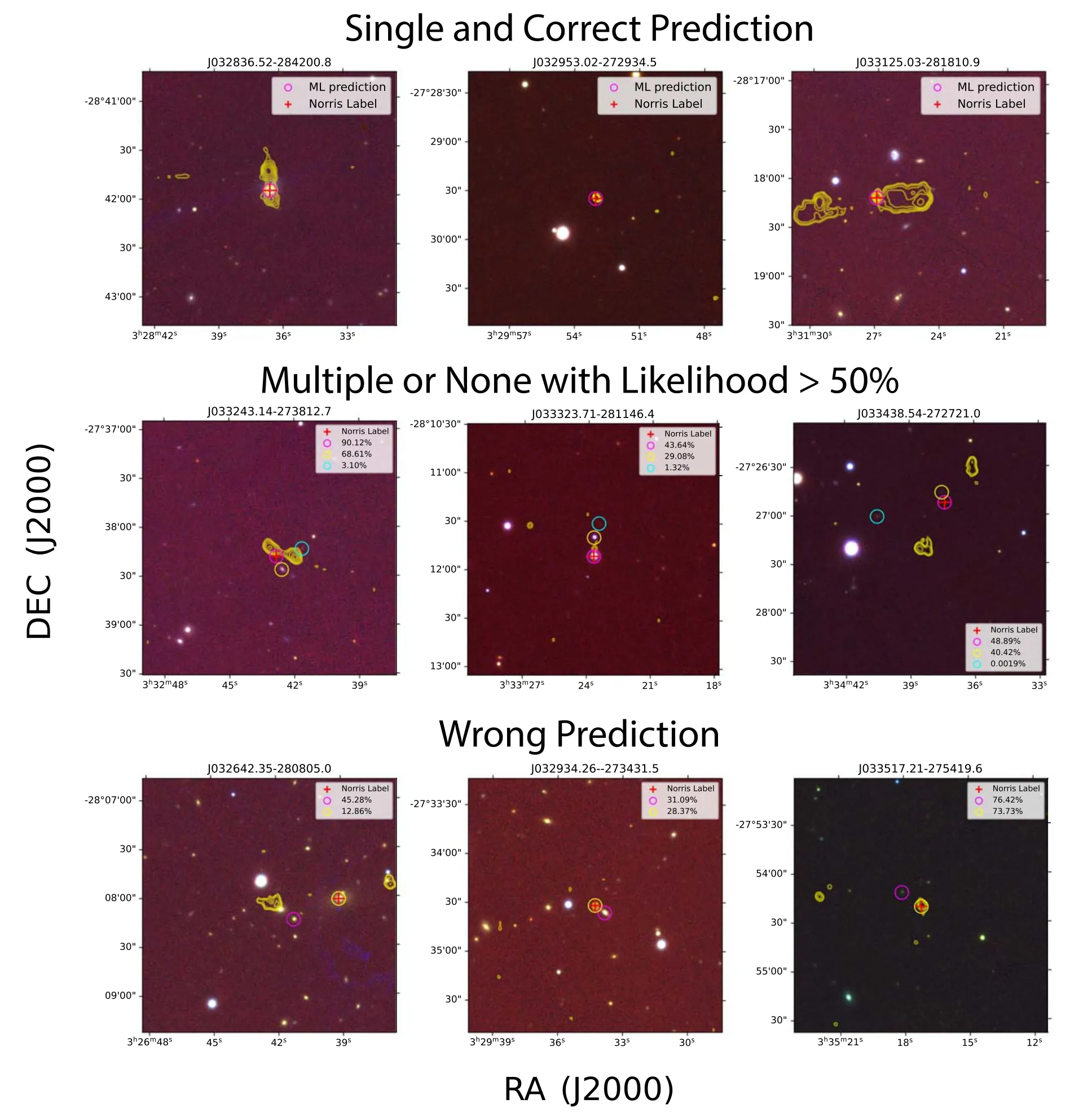
Figure 8.Examples of the model’s prediction results.The optical Pan-STARRS images are overlaid in each panel with VLASS radio contours.The red cross in each panel labels the true host identified by Norris et al.(2006).The magenta circles are the best possible or prime host candidates predicted by our model.The blue and yellow circles indicate other optical sources our model assigns a high likelihood of being the host of the radio emission.The top row shows three cases with prime host candidates that are consistent with the experts’labels.Among the 71 testing samples,the majority(58)of systems are in this category.The middle row shows the cases where multiple sources (leftmost panel) or none of the sources (middle and right panels) have a likelihood ＞50%.The optical source with the highest likelihood is assigned as the best possible candidate for the host.In 10 cases in the testing sample in this condition,our model successfully predicts the correct host in all of the systems.The bottom row shows the three cases in which the host is wrongly predicted.

Of the 71 testing sample systems,61 have only one positive host candidate in the field,including 58 correct predictions and three incorrect predictions.For the remaining 10 objects,multiple possible host candidates were assigned.For example,in the case of J33243.14−273812.7,the model predicted two out of the 17 optical sources nearby as positive host candidates as shown in Table 3.The optical source with the highest likelihood matches the true host in this case.

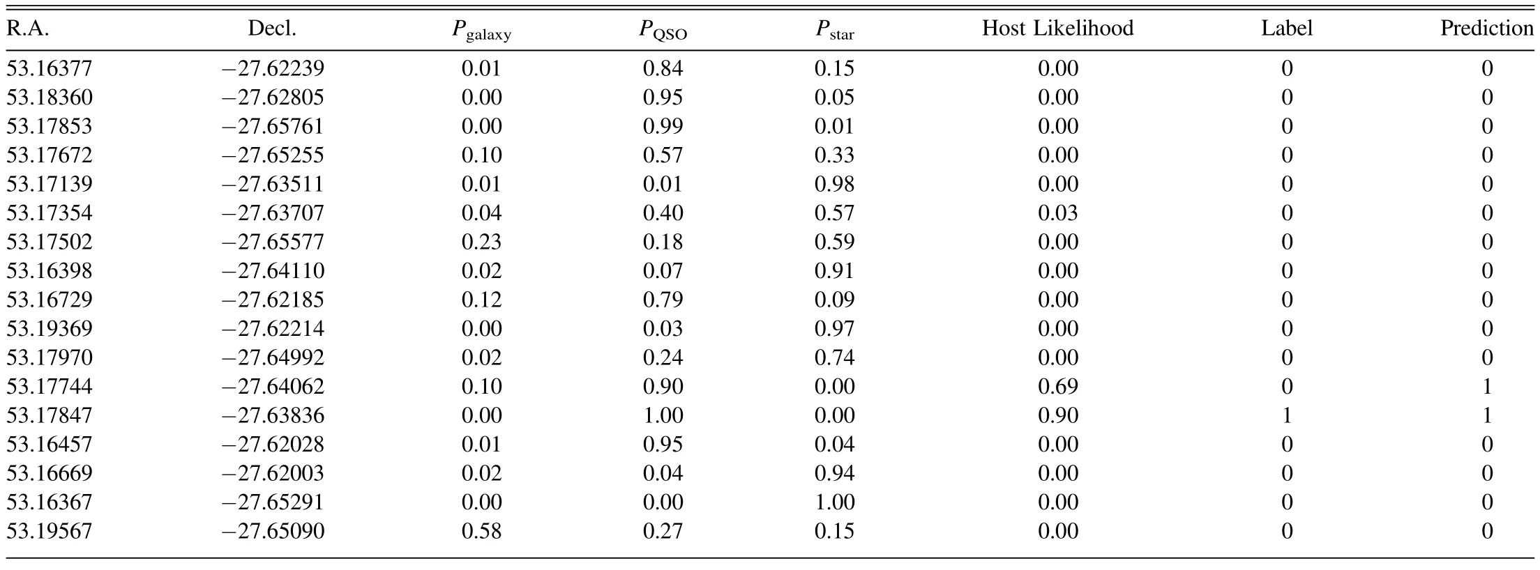
Table 3Optical Host Likelihood in the Field of Radio Galaxy J33243.14-273812.7—an Example with Multiple Positive Host Candidates Predicted

We have carefully examined the three cases(the bottom row of Figure 8)where our model has made inconsistent predictions with the experts’ visual inspection results.In the bottom left case there are two major radio components in the field of view of this radio cutout.Norris et al.(2006) identified the optical source in between the two radio components as the host;our model also identified it as the second most likely host.However,judging from the shape of the central radio component,it is also possible that the optical source on the edge of the radio contour is the central radio emission’s host,while the other radio component near the border of the image field of view is unrelated.The case of VLASS J033517.21-275419.6 (bottom right in Figure 8) is similar.Norris et al.(2006) treats the right source as emission from the AGN with the left source unrelated,or a jet,while our model treats them both as jets.This leads to the difference in the prediction result.As for the middle case of the bottom row in Figure 8,the optical source that is labeled as the host of this radio component is much fainter than the nearby one circled in magenta by the model.That is probably why the model considers this source the most likely,though no source is identified as more likely than not.From these limited cases,we might predict that figuring out if a radio component near the edge of the image field of view is an chance alignment or a member of this radio source has a profound compact on the model’s prediction performance.

In conclusion,our model made three wrong predictions out of the 71 Norris samples,making its overall accuracy ≈95.5%.

5.Discussion

5.1.Comparison with Other Automation Methods

The likelihood ratio (Sutherland &Saunders 1992;McAlpine et al.2012;Williams et al.2019;Kondapally et al.2021) method is commonly used to cross-match between unresolved radio sources and sources in other bands.This limits its usage in high angular resolution radio surveys.Fan et al.(2015) proposed a geometric model representing a threecomponent radio galaxy and used Bayesian hypothesis testing to achieve reliable associations.However,the simple straightalignment assumption for the three radio components limits its applicability in systems with complex morphologies.Fan et al.(2020) improved the method by allowing the core and two lobes to form an angle,mitigating the limitation.Weston et al.(2018)introduced the color of sources as a second parameter of the likelihood ratio function,further improving the performance in cross-matching non-extended radio sources.

Compared to these non-machine learning-based automation methods,our machine learning approach can be easily applied to both resolved and unresolved radio sources.In addition,our method does not rely upon simplifying assumptions about source morphology that limit the applications of the threecomponent approach.Last but not least,our method performs better in predicting the host for a radio galaxy than the nonmachine learning methods discussed above.

Before this work,little was done on radio galaxy host identification using machine learning except for work such as that by Alger et al.(2018).In that work,a two-layered CNN was used to extract features of radio sources.The authors manually selected an optical feature vector with a length of 10 for the sources in the optical host candidate catalog.In our case,we extracted optical features using another CNN based on Resnet-18 for the optical source classification,which minimized human involvement in the process.To increase the efficiency in host identification,we imposed the optical source classification with CNN beforehand.This procedure is proved to be as effective as the relative positions of the optical sources to the radio components.Nevertheless,we included the relative location information to improve the correct prediction rate.

5.2.Centroid and the Geodesic Center to Identify the Core of a Radio System

The radio emission of extended radio galaxies originates from collimated jets of relativistic electrons ejected in opposite directions from the central engine of the AGN.The basic symmetry of the ejection process means that the radio core where the AGN resides should be at,or near,the geodesic center of a graph constructed from the trajectories of the ejected mass.The same should hold for graphs constructed from the projected images of the jets.Thus the location of the host has a higher chance of being around the center along the radio structure,even though the radio structure of a radio galaxy usually has a certain degree of asymmetry.A simple approach is to find the geometric centroid using the flux density values as weights to determine the mean position on the radio structure.This method is robust and easy to implement.However,for the radio sources with bent structures,such as C-shaped radio galaxies,the geometric central location can fall outside radio structures and be further away from the real location of the host galaxies.Another approach is to find the geodesic center of the object.This geodesic center has a minimized maximum distance from all other points along the bent structure.Figure 9 shows two examples in this case.Both the geodesic center and the geometric centroid point in an image of a bent-typed radio galaxy are displayed.The prediction of the host galaxy can be enhanced by implementing the geodesic center information into the model for the C-shaped radio galaxies.

Figure 9.The geodesic center versus geometric centroid.The core position of bent-typed radio galaxies can be correctly located by the geodesic center,while the centroid points in such cases fall outside the shape.

5.3.Limitations of Our Method and Future Improvements

Although our model has achieved high accuracy in identifying hosts of radio components,there are still some limitations in our work.Most significantly,the small size of the training and testing samples used in training our machine could be inadequate for a generalized host galaxy identifier for all the radio galaxies in different radio surveys.

Currently,our model only includes the geometric centroid,which is robust for most radio galaxies.For C-shaped galaxies,however,the geometric centroid can fall far outside the radio structure,leading to failed predictions.The geodesic point could play an important role in identifying the radio core for C-shaped galaxies,such as the narrow-angled tail and the wideangled tail systems.For radio sources with multiple nonconnected components,however,or with only one component existing in the image,the geodesic center will not work and the geometric centroid of the shape is a better alternative.Thus,including the geodesic center would be an improvement,but it should only be included for radio galaxy systems with specific types of radio morphology.This improvement can be implemented in our future machine learning models.

Another problem arises for sources near the detection limit of the survey.If the radio galaxy consists of multiple disconnected components,not all of which pass the detection limit of the catalog(usually 5σ),then the source will appear to only have one highly asymmetric component,making both centroid techniques non-viable.There is an inherent trade-off in how much effort to put in characterizing sources that currently have a low signal-to-noise ratio.On the positive side,they are usually the most numerous sources,by far.On the negative side,they will likely be high signal-to-noise ratio sources once the next survey is done.

Even with high accuracy,our model can be further improved for more sophisticated applications.For example,a more meticulous radio morphology classifier can help us to revise the structure of our network assembly to better identify the host galaxies around the radio complex in “irregular” types of radio galaxies.The more distinct types,such as X-shaped,Z-shaped or C-shaped radio galaxies,can be recognized as demonstrated by Ma et al.(2019) using a CNN-based autoencoder.In addition,a better prediction of the possible host location can significantly improve the effectiveness of our model.As discussed in Section 5.2,the geodesic center can better determine the location of the radio cores in C-shaped radio galaxies.Although C-shaped radio galaxies are just a small proportion of all the radio sources,our model can be revised to accommodate these morphology-specific improvements.

6.Summary

We presented a deep learning-based approach for identifying the hosts of extragalactic radio components.The objects labeled in the RGZoo project,with their visual inspections by the citizen scientists,are treated as authentic in our training set.Their selection of hosts from the optical sources in the field of radio galaxy system is considered as the positive training set,while the rest of the nearby optical sources is the negative set.We take the catalog of expert-identified hosts of radio galaxies made by Norris et al.(2006)as the testing sample.We use the radio imaging data from an ongoing radio sky survey(VLASS),which has an angular resolutionthat is comparable to the seeing-limited Pan-STARRS optical sky survey data,as the radio data set for training and testing our machine learning model.

We tested our model on the radio galaxy sample from the CDFS field of ATLAS.Out of the 71 radio sources in the testing set detected by both ATLAS and VLASS in this field,our model only predicted the incorrect host for three of them.Thus,the model’s overall accuracy is greater than 95%.Compared to other work on the radio galaxy host identification problem,our method is more effective in identifying the hosts of radio galaxies with extended radio structures.Our optical source classification model achieves an overall accuracy of over 98%.Making the outputs of the optical source classification as inputs to the cross-identification network boosts the efficiency and accuracy of the final results.

We further investigated the method to determine the core location using the geodesic centers of the radio emission of a radio galaxy.This approach can better suggest the location of the host galaxy in the complex radio structure such as that in the C-shaped radio galaxies and can be incorporated into existing methods,including the radio host identification model discussed in this paper.These multi-band cross-matching tools can provide valuable information about the host galaxies of the extragalactic radio systems discovered in the ongoing radio sky surveys such as VLASS,Evolutionary Map of the Universe(Norris 2011) and the LOFAR Two-meter Sky Survey(Shimwell et al.2017),as well as in the future radio sky surveys by new generation facilities such as SKA and ngVLA.

Acknowledgments

This work was supported by grants from the National Natural Science Foundation of China (Nos.11973051,12041302).Sean Lake was funded by Chinese Academy of Sciences President’s International Fellowship Initiative.Grant No.2019PM0017.The authors acknowledge the Radio Galaxy Zoo Project builders and volunteers listed in full at http://rgzauthors.galaxyzoo.org for their contribution to RGZ data set and labels used in this paper.We also acknowledge the National Radio Astronomy Observatory(NRAO)for providing the source of the data for this research.NRAO is a facility of the National Science Foundation operated under cooperative agreement by Associated Universities,Inc.This work made use of the Swinburne University of Technology software correlator,developed as part of the Australian Major National Research Facilities Programme and operated under licence.This publication also makes use of data products from theWidefield Infrared Survey Explorer(WISE),which is a joint project of the University of California,Los Angeles,and the Jet Propulsion Laboratory/California Institute of Technology,funded by the National Aeronautics and Space Administration.In addition,we acknowledge the help from The Pan-STARRS1 Surveys (PS1).PS1 public science archive have been made possible through contributions by the Institute for Astronomy,the University of Hawaii,the Pan-STARRS Project Office,the Max Planck Society and its participating institutes,the Max Planck Institute for Astronomy,Heidelberg and the Max Planck Institute for Extraterrestrial Physics,Garching,The Johns Hopkins University,Durham University,the University of Edinburgh,the Queen’s University Belfast,the Harvard-Smithsonian Center for Astrophysics,the Las Cumbres Observatory Global Telescope Network Incorporated,the National Central University of Taiwan,the Space Telescope Science Institute,the National Aeronautics and Space Administration under grant No.NNX08AR22G issued through the Planetary Science Division of the NASA Science Mission Directorate,the National Science Foundation grant No.AST-1238877,the University of Maryland,Eotvos Lorand University (ELTE),the Los Alamos National Laboratory,and the Gordon and Betty Moore Foundation.This research has made use of the VizieR catalog access tool,CDS,Strasbourg,France.The original description of the VizieR service was published in A&AS 143,23.

ORCID iDs