Machine learning method to predict dynamic compressive response of concrete-like material at high strain rates

Xu Long ,Ming-hui Mo ,Tin-xiong Su ,Yu-ti Su ,Meng-ke Tin

a School of Mechanics, Civil Engineering and Architecture, Northwestern Polytechnical University, Xi'an, China

b School of Civil Engineering, Liaoning Petrochemical University, Fushun, China

c Beijing Microelectronics Technology Institute, Beijing, China

Keywords: Deep learning LSTM network GA-BP network Dynamic behaviour Concrete-like materials

ABSTRACT Machine learning(ML)methods with good applicability to complex and highly nonlinear sequences have been attracting much attention in recent years for predictions of complicated mechanical properties of various materials.As one of the widely known ML methods,back-propagation(BP)neural networks with and without optimization by genetic algorithm (GA) are also established for comparisons of time cost and prediction error.With the aim to further increase the prediction accuracy and efficiency,this paper proposes a long short-term memory (LSTM) networks model to predict the dynamic compressive performance of concrete-like materials at high strain rates.Dynamic explicit analysis is performed in the finite element(FE)software ABAQUS to simulate various waveforms in the split Hopkinson pressure bar(SHPB)experiments by applying different stress waves in the incident bar.The FE simulation accuracy is validated against SHPB experimental results from the viewpoint of dynamic increase factor.In order to cover more extensive loading scenarios,60 sets of FE simulations are conducted in this paper to generate three kinds of waveforms in the incident and transmission bars of SHPB experiments.By training the proposed three networks,the nonlinear mapping relations can be reasonably established between incident,reflect,and transmission waves.Statistical measures are used to quantify the network prediction accuracy,confirming that the predicted stress-strain curves of concrete-like materials at high strain rates by the proposed networks agree sufficiently with those by FE simulations.It is found that compared with BP network,the GA-BP network can effectively stabilize the network structure,indicating that the GA optimization improves the prediction accuracy of the SHPB dynamic responses by performing the crossover and mutation operations of weights and thresholds in the original BP network.By eliminating the long-time dependencies,the proposed LSTM network achieves better results than the BP and GA-BP networks,since smaller mean square error (MSE) and higher correlation coefficient are achieved.More importantly,the proposed LSTM algorithm,after the training process with a limited number of FE simulations,could replace the time-consuming and laborious FE pre-and post-processing and modelling.

1.Introduction

Concrete is one of the most widely used materials in the structural engineering because of its low price and fabrication convenience.During the long-term service,concrete structures may experience high-strain-rate dynamic loadings such as earthquakes,explosions or impacts.It is greatly expected to enhance the mechanical behavior of concrete by prolonging the life of concrete structures for structural safety.According to extensive studies in recent decades,the split Hopkinson pressure bar(SHPB)is widely accepted to achieve more accurate controls and broader ranges of strain rate under dynamic loading conditions [1-4],compared with the drop-weight experiments [5,6]and hydraulic servo experiments [7-11].With the development of SHPB testing technique,it is essential to establish identifiable and accurate wave shapes of incident,reflect and transmission waves which represent the dynamic responses of materials subjected to different strain rates.Therefore,accurate and efficient determinations of waveforms are crucial to evaluate the dynamic performance of concretelike materials.As preparations prior to SHPB experiments,an airimpact test without specimens is usually conducted with laborious adjustments to ensure that incident and transmission bars are aligned.In addition to time-consuming SHPB experimental procedures,recent studies show that some potential problems need to be concerned in SHPB experiments with large-diameter bar for concrete materials such as lateral confinement effect,evolution of cracks,and viscosity effect[9].The conventional SHPB experiments are difficult to alleviate these problems,so finite element (FE)simulations and theoretical approaches are more advantageous due to the lack of requirements for experimental conditions.

Because of its great advantages for nonlinear mapping,selflearning,and robustness,ANN technology has been widely employed to predict the mechanical characteristics of materials and structures as a common type of machine learning.Deep learning and ensemble models have more complicated network architectures than typical ANN algorithm.In particular,the ensemble model is composed of several independently trained models whose predictions are integrated to some extent to make the final prediction.These algorithms make it difficult to comprehend and analyze dynamic response predictions for concrete-like materials that are subjected to high strain rates.Rumelhart and McClelland[12]firstly developed the back-propagation (BP) algorithm on the basis of ANN.The proposed BP algorithm significantly promoted the development of ANN-based models thanks to its outstanding capacity of arbitrary complex pattern classification and excellent multi-dimensional function mapping.Goh [13]applied BP algorithms to analyze the sand data from calibration chamber tests and also predict the ultimate load capacity of driven piles.Wang et al.[14]conducted SHPB experiments to study the dynamic behavior of Ti-Ni alloy and predicted the dynamic response by establishing a BP algorithm without any pre-assumption about the constitutive model.Because of rapid development of hardware and software in computer technology,the BP algorithm regained intensive attentions and applications in recent years.Nevertheless,some demerits of the BP algorithm are also noteworthy such as slow convergence speed,prone to be stuck in local minimum,uncertainty of hidden layer neuron and so forth [15,16].Genetic algorithm (GA) is a computational model of biological evolution process that simulates the natural selection and genetic mechanism according to the Darwin's theory of biological evolution.Whitley[17]attempted the GA to solve the shortcomings of BP algorithm by optimizing initial network parameters.The combination of GA and BP network has been successfully used in the areas of structural member analysis,fault diagnosis and strategy evaluation [18-21].

To achieve superior prediction capacity of machine learning(ML),advanced deep learning (DL) models were developed based on ANN framework,such as convolutional neural networks(CNN),recurrent neural networks (RNN),and graph neural networks(GNN).However,few works used DL models for predicting mechanical properties of concrete[22,23].Tanyildizi et al.[24]studied the mechanical properties of concrete containing silica fume exposed to high temperatures with LSTM networks (i.e.,a typical RNN model in DL) to prove this approach has a great potential in civil engineering applications.Deng et al.[25]used a CNN model to learn and predict the compressive strength of recycled concrete.Their predictions demonstrated the advantages of DL modelling with higher precision,higher efficiency and higher generalization ability compared with the traditional ANN models.Zhang et al.[26]developed the least-squares support-vector machines (LS-SVM)model to analyze the soil-concrete interfacial shear strengths considering the effects of initial moisture contents,initial dry densities and normal stresses of soils.To predict the surface chloride concentrations in concrete containing waste material,Ahmad,et al.[27]used gene expression programming(GEP),decision trees(DT),and ANN.Additionally,Ahmad,et al.[28]presented the applications of DT,ANN and gradient boosting (GB) to predict the compressive strength of concrete at high temperatures.Farooq et al.[29]made a comparative study by ANN,GET and SVM algorithms for predicting the compressive strength of self-compacting concrete codified with fly ash.Individual and ensemble algorithms were used to predict the mechanical properties of concrete,with ensemble learning models having more favorable features and providing better results than individual learning models[30,31].It should be noted that compared with traditional ANN models,these DL-based models have more complex structures that enable better predictions but at more time cost.Furthermore,few studies in the existing literature are carried out based on ML methods to predict the dynamic behavior of the concrete-like materials at high strainrate.

In this paper,dynamic compressive responses of concrete at high strain rates are predicted using different ANN-based and DLbased models.Validated FE models are utilized in Section 2 to perform extensive impacting cases to generate incident,reflect and transmission waveforms in SHPB experiments.On the basis of BP algorithm as a typical ANN-based model,Section 3 proposes a framework for the GA optimized BP algorithm to predict the dynamic behavior of the concrete-like materials with more simplified network structures and fewer hidden layers.As a special DL model,LSTM has an improved RNN structure with the ability to remember or discard data,which is proposed for the relationship predictions between sequential arrays of dynamic responses and time histories.The proposed ML models are trained to establish the nonlinear mapping relations between incident and reflect waves and between incident and transmission waves,respectively.The merits of different ML models are compared and summarized with quantitative comparisons of prediction errors in Section 4.

2.Modelling for dynamic response of concrete-like material using SHPB

As shown in Fig.1,the whole SHPB setup usually includes strike bar,incident bar,transmission bar,waveform shaper and strain gauge.The strain gauges record the strain responses of incident and transmission bars during the whole impact process.The strain responses εiand εrare measured from the strain gauge attached on the incident bar before and after the impact to specimen.Apparently,the directions of incident wave and reflect wave are opposite.The strain response εtto represent the transmission wave is measured from the strain gauge attached on the transmission bar,which is greatly related with the strain responses εiand εrfrom incident and reflect waves at the same time history.

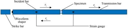
Fig.1.Schematic diagram of SHPB setup.

Because of different ways for data processing to ensure the dynamic force equilibrium at both end surfaces of concrete-like specimens,the dynamic behavior of concrete-like materials can be processed by two-wave and three-wave methods.According to the two-wave method,the multiplication of the stress at one of specimen end surfaces by twice and thus calculation error can be found especially for concrete-like specimens.Compared with the two-wave method,the three-wave method can strictly meet the dynamic force equilibrium through the superposition of three waveforms and thus reduce the calculation error.Additionally,the three-wave method is superior in the calculation of dynamic strain rate,which is thus selected in this study to describe the relationship between stress and strain at high strain rates.

To satisfy the force equilibrium,Eq.(1)-Eq.(3) are provided to perform data analysis of SHPB experimental results.

where εsis the strain of the material specimen,and the dot on top of the εsrepresents the derivative of the strain with respect to time.LsandAsare the specimen length and cross-sectional area,respectively.Besides,some SHPB related paraments are defined as follows:C0is the wave velocity of the bar as defined by (Eb/ρ)0.5,τ is the time of during the process;Eb,the elastic modulus of the bar,ρ is the density of the material of the bar,Abis the area of the bar.Regarding stress,σ1and σ2are the stresses on the front and end surfaces of the material specimen,and σsis the stress in the specimen.By assuming σ1equal to σ2,the stress wave can be considered one-dimensional in the elastic bars,and the specimen stress and strain are uniform in the axial direction of the specimen.

Quite a number of constitutive models have been adopted in SHPB simulations,such as Drucker-Pager [32,33],and Holmquist-Johnson-Cook (HJC) [1,2].In this paper,the simulations are performed by using the Drucker-Prager model in ABAQUS/Explicit(2017) with the element type of C3D8.The geometric parameters and material types of material specimen and the bars of SHPB simulations are listed in Table 1,which has been adopted in the previous studies about dynamic mechanical properties of concrete materials[34,35].The material parameters of the steel for the bars and the mortar for the specimen are listed in Table 2.More information about the constitutive model and the FE model validation can be found in the recent paper by the authors [36].Meshsensitivity analysis has been conducted by trial simulations to find an optimal mesh scheme(i.e.,1 mm for the characteristic size of material specimen and 10 mm for the characteristic size of material steel incident and transmission bars) which balances the computational accuracy and cost.

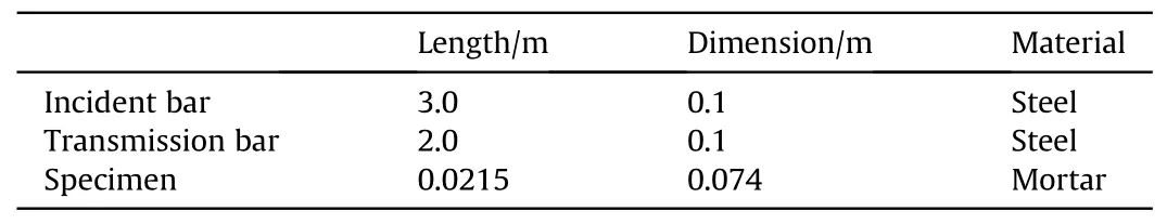
Table 1 Geometry and material of the specimen and bars in SHPB simulations.

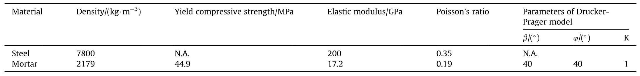
Table 2 Material parameters in the established FE model.

The dynamic increase factor (DIF) is defined as the ratio of the peak strength in SHPB experiments and the quasi-static ultimate strength to determine the dependence of dynamic strength ofmaterials on strain rates.Fig.2 describes the quasi-static uniaxial stress-strain relationship of concrete [37].As the peak strength is 44.9 MPa at a quasi-static state,the DIF can be obtained by dividing the predicted dynamic peak stress in MPa by 44.9 MPa.The friction between the bars and the material specimen plays an important role in the strength hardening of the concrete-like materials.Li and Meng [38]found that when the friction was greater than 0.2,the DIF of concrete-like materials was significantly enhanced.Also,the friction constrained the lateral motion of specimens.Since the friction between the specimen and bars is challenging to be determined,the value of 0.2 is assumed in this study to emphasize the strain-rate effect by dynamic deformation rather than by friction.

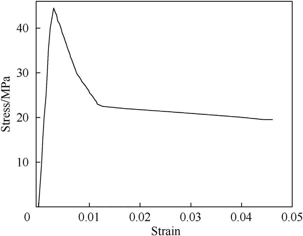
Fig.2.Quasi-static uniaxial compressive stress-strain curve of concrete.

3.Proposed ML models trained using FE predictions

3.1. BP model

The major interest of this works is to propose outstanding networks with superior advantages for predictions of dynamic responses of concrete-like materials.As a control model,the conveniently available ANN-based BP model is selected in this study.The ANN-based BP model usually consists of input,hidden and output layers to realize the function estimation,model recognition and data compaction.In the training process,the values of weights and thresholds are adjusted to minimize the error between the actual output and the predicted output using the function based on the Delta rule.This process is repeated until the output error is minimized to satisfy the allowable tolerance.The BP algorithm as proposed by Rumelhart and McClelland [12]is expressed as

wherexiis the parameter of input layer,wijis the weight of neurons,ajis the threshold of hidden layer,andHjis the target output.Regarding the activation functionf,common nonlinear activation functions includelogsig,tansig,purelin,etc.The hyperbolic tangent functiontansigis selected in this study to minimize the mean square errors,which is written as

According to the input-output sequence (x,H) of the network,the node numberlin the hidden layer is determined by following the empirical formula Eq.(6)and Eq.(7)with the node numbernin the input layer and the node numbermin the output layer.In addition,the constantcis within the range from 1.0 to 10.

The whole training process can be divided into two steps,i.e.,feed-forward of the input training pattern and the adjustment of the weights by error.

(a) Data propagation forward from the input to the output.The prediction values of each layer are calculated by

wherenethiis the sum of dataXhi-1after matrix operation,Whiis the weight of neurons between different layers,biis the threshold of each layer,andXhiis the prediction output of each layer.It should be noted that there are three layers with the layer number denoted byi.That is,the subscripts 1,2,and 3 represent the input,hidden and output layers,respectively.

(b) Backward propagation of errors to adjust the weights in all layers.The errorehibetween the prediction valueXhiand the target valueYhiin each layer can be expressed in Eq.(10).The network weightsWhiandbican be updated by Eq.(11) and Eq.(12) with the learning rate of η.Moreover,Wh3andb3represent the weight and threshold between the hidden and output layers as given in Eq.(11) and Eq.(12).

When the error meets the accuracy requirement,the learning process is terminated and the corresponding neural network is output.If accuracy requirement is not satisfied,one should iterate in steps (a) and (b) until the errorehiis within the allowable tolerance.The detailed learning parameters are described in Section 4.

3.2. BP model optimized by GA

The GA randomly generates numerous sets of data to simulate the population in the process of biological evolution.Each data set is called an individual,and GA selects the optimal individual by constantly changing individual characteristics.Meanwhile,the fitness function is used as the target to guide the GA optimization.As a result,GA could optimize existing algorithms.In essence,GA consists of three parts,that is,selection operation,crossover operation and mutation operation.After these operations,the optimal individuals can be traced by the fitness function.More importantly,the GA is portable and implemented to any network.The GA optimized BP model is proposed to further improve the prediction accuracy.The prediction error of the GA-BP network is selected as the fitness value.The mean square error (MSE) is adopted in Eq.(13) as the fitness function to highlight the critical strain waveforms during the impact process.

whereyiis the prediction by FE simulations,ypreiis the prediction by the algorithm,andnis the data size.As theMSEis defined by the average squared difference between the estimated and actual values,a smallerMSEvalue represents greater consistency between the two groups of data.

(a) Coding and group initialization.Real number coding is adopted.Each connection weight is directly represented by a real number,and the string lengthLDNA=m×l＋l＋l×n＋n(wheremis the number of input nodes,lis the number of hidden nodes,andnis the number of output nodes).It is worth mentioning thatLDNAis usually expressed as an individual in GA.The code is linked into a long string in a certain order,and each string corresponds to a set of network connection weights.A distribution of network weights is expressed by an individual.

(b) Calculation of each individual.Fitness function is used to check the quality of the individual which is a real string containing the weight and threshold of the neural network in this paper.By introducing weights and thresholds in individuals into the BP network,the selection of fitness function is crucial to optimal selection.With all the individuals calculated by the fitness function,the average fitness is traced and thus the GA could select the best individual in the whole population.The fitness function selected in this paper is written in Eq.(13).With the GA continuous accumulation,the function accuracy corresponding to the moderate function is continuously improved,and finally the trained network can meet the requirements of the algorithm.

(c) Selection operation.The probability of selecting an individual in this operation is proportional to the fitness of the individual [39].In general,the better the fitness value of individuals,the greater the selection probability is.First,the fitness functionMSEof all individuals is calculated,and then the selection probability is calculated according to Eq.(14)and Eq.(15).For the individualLDNAi,the fitness value is set asFi,kis a constant,piis the selection probability.And a total ofNselection operations are performed,the numberNis the initial population size.

(d) Crossover operation.As crossover operator is the most important operation among the three operations of genetic algorithm,different new individuals will make the individuals as fertile as possible to be generated through crossover,and the new individuals are different from the previous generation.Therefore,multiple crossover operation will traversal all the solution,which facilitates finding an optimal global solution.With a certain probability,the DNA of the two selected individuals is exchanged to produce two entirely new individuals.This is the basic operation of crossover.The crossover operation at thejposition betweenkth individualakandlth individualalis

whereba random number in the interval [0,1].

(e) Mutation operation.The mutation operation can increase the population diversity and thus greatly reduce the probability of the network falling into the local minimum.In this method,one or several individuals are randomly selected as mutation objects.At a position in the real number string of the randomly selected individuals,mutation object is performed according to Eq.(18) and Eq.(19).

whereamaxandaminare the upper and lower bounds ofaij,gis the current iteration number,Gmaxis the number of evolutions,andris a random number in the interval[0,1].All the above operations are conducted only when the random numberrgenerated by the computer in the interval [0,1]is larger than the mutation probability.The operations for GA process crossover and mutation are illustrated in Fig.3.

Fig.3.Diagram of GA process crossover operation and mutation operation.

As a flowchart,Fig.4 shows that the GA is combined to optimize the weight and threshold values in the training process of the BP algorithm.The weights and thresholds are arranged in a real number string in step(a)of Section 3.2 to simulate the DNA chain in the genetic process.The GA optimization was completed with the number of populations of a certain size and also the corresponding crossover and variation coefficients.The total number of the whole individuals is 17,856.The weight and threshold values between the input and the hidden layers are 8785 and 35,respectively,while the weight and threshold values between the hidden and the output layers are 8785 and 251,respectively.Furthermore,the crossover probability is 0.1,and the mutation probability is 0.1.After optimization,the optimal initial thresholds and weights are determined as the initial parameters of BP network.More discussions about parameters will be explained in detail in Section 4.

Fig.4.Flowchart of the proposed GA optimized BP algorithm.

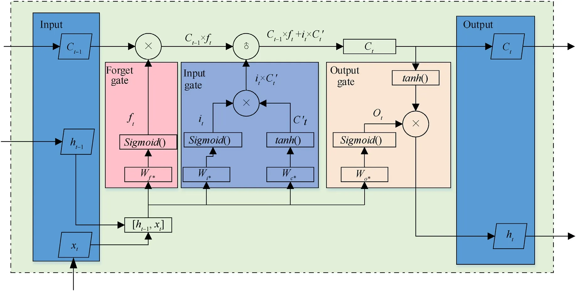
Fig.5.Flowchart of the proposed LSTM network.

3.3. LSTM network

The LSTM network is proposed to eliminate the disadvantage of the original RNN model due to long-time dependencies which means that the predictions for the current output require the information stored a long time ago.Unlike the original RNN model,a memory block controlling the data store is enriched to record the weights and thresholds of all previous learning samples.This memory block controls both incoming and outgoing data through input,forget,and output gates.At the given timet,LSTM has three inputs (i.e.,the current input valuext,the hidden stateht-1of the previous cell,and the previous cell stateCt-1)and two outputs(the current hidden stateht,and the current cell stateCt).More details of the LSTM parameters will be explained in Section 4.

(a)Forget gate.As one of the gates to control the cell stateCt-1in the LSTM network,the forget gateftdetermines the cell stateCtfrom the previous moment is retained to the current moment,which is given as

whereWf,WfhandWfxare the weight matrices in forget gate,andbfis threshold.Besides,ht-1andxtare the previous output value and the current input data.

(b)Input gate.The next important control part of this algorithm is the input gate,which determines the current network inputxtsaved in the cell stateCtand can be expressed by Eq.(22)-Eq.(24),whereWiandWcare the weight matrices of the input data and cell state value in input gate,bcandbfare thresholds.The current cell stateCtis thus obtained.

(b) Output gate.As the last control part of this algorithm,LSTM uses the output gate to control the cell stateCtthat is exported to the current output valueht.It can be expressed by Eq.(25)and Eq.(26),whereOt,Wo,boare the output gate value,weight matrices and thresholds in the output gate.

All the three gates work together to output the cell stateCtand the output valueht,the gradient disappearance problem in the original RNN model due to long-time dependencies can be resolved.

4.Results and discussions

As a representative case,the SHPB experiment subjected to the incident wave with the peak stress of 160 MPa is simulated by FE simulations and the corresponding dynamic responses discussed in Fig.6.The incident stress is directly applied on the free surface of the incident bar,which is further simplified by Zhang et al.[40]to ensure the numerical convergence.Specifically,the peak stress σiof the incident wave is smoothly transited by an exponential-based function by Eq.(27),where σ is the stress in the incident bar with the unit of MPa and τ is the time with the unit of μs.The applied stress wave lasts for 500 μs,and the simulation covers the process up to 1400 μs to capture the whole deformation history in SHPB simulations.

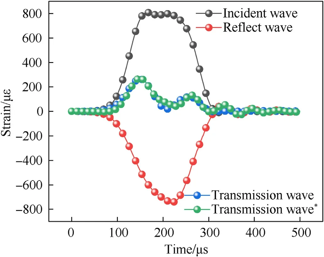
Fig.6.Typical strain history of SHPB experiment by FE simulations.

Fig.6 shows the typical strain history of incident,reflect and transmission waves under the incident wave with the peak stress of 160 MPa.After a wave shift processing,these waves meet the requirements at the same starting time of the waveforms in Eq.(1)-Eq.(3).By the summation of the incident and reflect waves in the same time duration,one more curve labeled as transmission wave*is given to examine whether the assumptions of SHPB experiments in Section 2 are satisfied in the process of impact simulation.It can be clearly seen from Fig.6 that the waveforms of transmission wave* and the transmission wave achieve good agreement.This indicates that the stress wave is propagated one-dimensionally,and the stress and strain are uniformly distributed in the axial direction of the specimen.

Different methods of determining the strain rate leads to different strain rates even based on the same set of experimental data.This may lead to the lack of objectivity in investigating the strain-rate effect of concrete-like materials.Therefore,it is important to reasonably determine the strain rates of concrete materials in SHPB experiments.European CEB [41]recommended a DIF formula for concrete in compression in the following form:

wherefcdandfcsare the unconfined uniaxial compressive strength in quasi-static and dynamic loading,respectively.γs=10（6.156αs-2）,αs=1/（5 ＋9fcs/fc0）˙εs=3×10-5s-1,fc0=10 MPa,andfcs=44.9MPa Based on Eq.(28),Fig.7 gives the predicted DIF distribution by the CEB formula along with a wide range of strain rate,which reasonably fits the SHPB test results by Malvern and Ross[42]and also verified by verified by Bischoff and Perry [43].

Fig.7.DIF comparison at different strain rates.

One DIF regression equation in Eq.(29) was proposed by Tedesco and Ross[44],in which the transition from the low strainrate-sensitivity to the high strain-rate-sensitivity occurs at a critical strain rate of 63.1 s-1.This transition strain rate is slightly higher than that regulated by the CEB formula in Eq.(28).

According to the comparisons in Fig.7,the predicted DIF of the concrete materials by the CEB formula is close to the values from the SHPB experiments reported by Zhang et al.[40].With the validated FE model and material properties in Section 2,more extensive simulations are conducted for 60 different loading cases with the incident peak stress ranging from 3 to 180 MPa with an increment of 3 MPa[45].The incident stress is applied based on Eq.(27).As observed in Fig.7,the predicted dynamic peak strengths by the FE simulations are significantly improved due to the significant increase of strain rate.The good agreement with other predictions and experiments confirms the accuracy of the FE simulations for predicting the dynamic behaviour of concrete-like materials at high strain rates.

Confirmatory factor analysis(CFA)aims to confirm a theoretical model using empirical data[46].To make the data more statistically meaningful,the Pearson correlation coefficient (R) and coefficient of determination (R2) are adopted in Eq.(30) and Eq.(31) in addition to theMSEas adopted by Botchkarev [47]in Eq.(13),which aims to objectively measure the correlation between predictions by FE simulations and the proposed networks during the impact process.

whereXiis the value calculated by FE simulations,Yiis the value predicted by networks,andNis the data size,andthe mean value predicted by networks.As theRvalue represents the linear correlation,it is generally believed that theRvalue of 0.8-1.0 can ensure a sufficiently high correlation between the two sets of data.R2should most be equal to 1.Similarly,the closer the value ofR2is to 1,the better the fitting degree of the regression line to the observed value is.On the contrary,the smaller the value ofR2is,the worse the fitting degree of the regression line to the FE simulation value is.

The FE predictions produce the data required by the input layer of the proposed ML algorithm,while the nonlinear mapping relations are expected to be established among incident,reflect and transmission waves by the proposed DL-based and ANN-based models.The wave duration is 500 μs,and thus there are 251 time nodes in total with an increment of 2 μs.The strain values on the incident and transmission bars are recorded to form the strain histories for the input layer.Thus,the incident waves and reflect waves or transmission waves are combined into a long sequence,and the 54 groups of learning samples are connected to form the LSTM algorithm training sequence randomly.The incident wave of the training sample is used as a set of sequence input to predict the corresponding reflect waves and transmission waves.The number of nodes in the hidden layer is 20,the solver is Adam,the maximum number of learning epochs is 35,and the initial learning rate is 0.005.To gain better predictions,the study varies the number of layers.Based on the comparisons listed in Table 3,it can be concluded that when the hidden layer is more than 3,theRvalue and theR2value are lower,and the ANN performance is insufficient to predict the waveforms in SHPB experiments.This means that more hidden layers do not significantly improve the ANN performance.On the other hand,more hidden layers result in more complex ANN structures,which make the optimization technique more difficult.As a result,the neural network model with a single hidden layer is chosen for optimization in this study.For ANNbased models,the BP network has a single hidden layer in which the node number is determined as 35 according to Eq.(6) and Eq.(7).

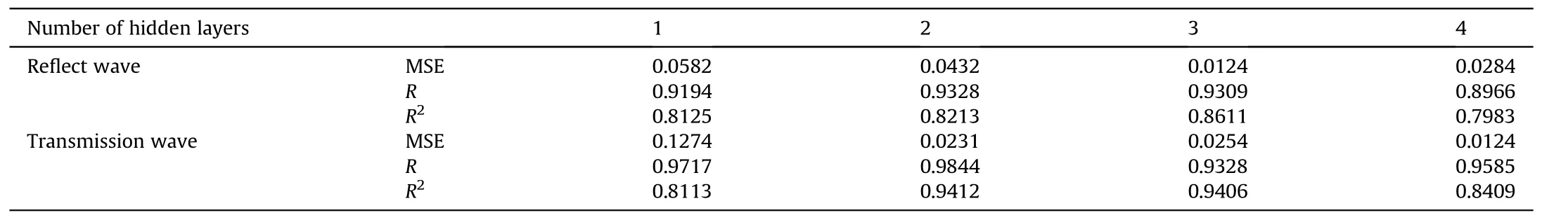
Table 3 ANN by varying the number of layers.

In the GA-BP multi-layer network,the input layer is the strain history of the incident wave,while the output layer is the strain histories of reflect and transmission waves.As explained in Section 3.2,the involved parameters in the GA architecture are given as follows: mutation iteration is 15,population size is 5,mutation probability is 0.1,and crossover probability is 0.1.Regarding the prescribed tolerance values,the maximum epochs of the BPnetwork are 500 for both reflect and transmission waves,while the tolerance ofMSEis 0.0001.In this study,the number of training and verification sets are determined as 54 and 6,respectively.Thus,the ratio of training set to verification set is 0.9:0.1,which can guarantee the rationality of ML model in a conventionally accepted standard.The greater process detail for training and validation sets of machine learning can be found in Fig.8.When any of the above tolerance values is satisfied,the training process is terminated with a numerical convergence.In order to clarify the data types in machine learning,the parameters of the database are listed in Table 4 for both training sets and validation sets.Meanwhile,the three machine learnings structural parameters are also described in detail.

Table 4 Parameters of the database with three ML models.

Fig.8.Performance of the training process.(a)and(b)MSE values along with the epochs for reflect and transmission waves;(c)and(d)Performance of GA optimization for reflect and transmission waves.

The values of loss functions for three networks and the fitness function during the GA optimization process are examined in Fig.8.Fig.8(a)and Fig.8(b)compare theMSEof the three networks with different epochs.It should be noted that all input and output data isnormalized so as to reduce the calculation time.Therefore,theMSEvalues in Fig.8 are during the training process rather than from FE predictions.Compared with ANN-based models,it can be clearly seen that the LSTM network has a much faster decreasing loss function and a smaller number of epochs.Moreover,theMSEvalues of the GA-BP network decreases faster than the original BP model,and also theMSEvalue is smaller than the original.The comparisons indicate that the prediction capacity of LSTM network is superior to that of ANN-based model even optimized by GA in terms of accuracy and epochs.Fig.8(c) and Fig.8(d) show the performance of the GA optimization for reflect and transmission waves.Because of GA,the BP network keeps improving with the continuous crossover and variation process of weights and thresholds.For the reflect wave,the GA optimal weight and threshold combinations of ANN models reduce theMSEvalues from 16.6 × 10-3to 7.5 × 10-3.Similarly,MSEvalues decrease from 21.8 × 10-3to 13.3×10-3due to the GA optimization for the transmission wave.It should be noted that when the value Generation=1,only acrossover operation of weight and threshold is carried out,so theMSEvalue is smaller than that of the original BP network.It is not difficult to see that GA can improveR2value and improve the neural network prediction performance.Besides,the LSTM algorithm has the bestR2value,indicating that LSTM algorithm has significant advantages for time sequential prediction.In addition,it should be noted that the ANN model terminates the training process if theMSEvalue of validation set increases for 200 epochs in a row,so theMSEvalue in the validation set appears to increase in Fig.8(a)and Fig.8(b).

In order to examine the predictions of the proposed three ML models,the predictions of the SHPB experiment subjected to the incident wave with the peak stress of 200 MPa as one of the validation datasets are compared with FE simulations and ML models in Fig.9.Fig.9(a) and Fig.9(b) show that the Pearson correlation coefficientRvalues of the three models are above 0.98.The LSTM network has theRvalues of 0.9948 and 0.9969 for reflect and transmission waves,which is sufficiently close to 1.0.For the ANNbased models,theRvalues keeps increasing with the increase of mutation iterations,reaching a value close enough to 1.0.Based on the comparisons in Fig.8,it can be found that compared with the original BP model,the BP neural network optimized by GA has better prediction accuracy on reflect and transmission waves as predicted by FE simulations.With the original BP network,the Pearson correlation coefficientsRof reflect and transmission waves are 0.9839 and 0.9583.After GA optimization,theRvalues are improved to be 0.9973 and 0.9856 for reflect and transmission waves,respectively.Therefore,the comparisons ofRvalues indicate that the predictions by the proposed models accurately reproduce the FE predictions,and the LSTM network can be accepted to be equivalent with the FE simulations.

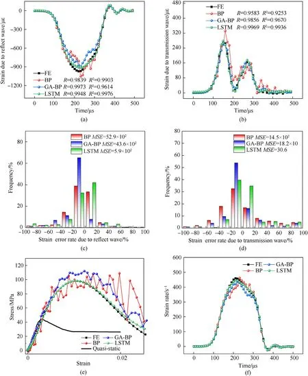
Fig.9.Comparisons of dynamic responses predicted by FE,LSTM,original BP and GA optimized BP models.(a)and(b)Strain history for reflect and transmission waves;(c)and(d)Error probability distribution for reflect and transmission waves;(e) and (f) Comparisons of constitutive behaviour for stress-strain curve and strain rate response.

In order to better evaluate the prediction accuracy of waveform correlation,all waveform values are processed by inverse normalization operation,and the unit is με.The error probability distributions are further compared in Fig.9(c) and Fig.9(d).The error rate of LSTM predictions is less than 20%,which is much better than the two ANN models.TheMSEvalues of reflect and transmission wave are 5.9×102and 30.6 with the unit με2,respectively.Due to the GA optimization,theMSEvalues of BP networks decrease from 52.9×102and 14.5×102to 43.6×102and 18.2×10 with the unit με2.It is worth mentioning that although the 20% error rate of reflect wave is much more than that of transmission wave,theMSEvalues show opposite results.Because theMSEvalue is mainly related to the error value rather than the error rate.For instance,when a large number of FE values in the transmission wave are close to 0,the error value is negligible but a large error rate is induced.Thus,the shape of the error frequency distribution is greatly affected.Fig.9(e)and Fig.9(f)describe stress behaviour for stress-strain curve and strain rate response.Apparently,the LSTM model has the best accuracy,and the GA optimization also improves the accuracy of BP network.

Table 5 summarizes the prediction accuracy and time cost for the impact simulation subjected to the incident wave with the peak stress of 200 MPa.All FE and ML analysis are fairly performed on a normal-sized computer(AMD(R)Ryzen(TM)3700X CPU@3.6 GHz CPU,32 GB RAM).Training time represents the time to complete the training process of the proposed network.It is apparent that the LSTM algorithm has advantages in terms of training time and accuracy for waveform in SHPB experiments.Despite of the cost of a shorter training time,the traditional ANN model has a greater prediction error.Besides,the GA optimization algorithm can improve the prediction accuracy but at greatly increasing time cost because of the update of more weights and thresholds.The comparisons in Fig.9 and Table 5 confirm that the proposed LSTM model is superior for predictions of dynamic responses in the time history compared with the ANN-based models.

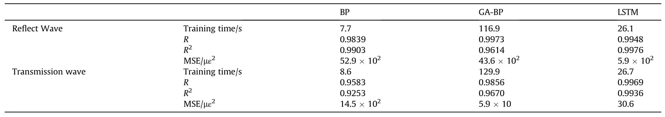
Table 5 Comparison of time cost and accuracy with three ML models.

5.Conculsions

This study proposed three ML models including the DL-based LSTM network and ANN-based BP networks with and without GA optimization to predict the dynamic responses in the time history for concrete-like materials subjected to high strain rates.Extensive FE simulations of SHPB experiments were conducted to scale up the sample number for ML training and validations.By the proposed ML models,the nonlinear mapping relations were reasonably established between incident,reflect,and transmission waves.Various statistical measures were used to validate the prediction performances.It was found that compared with the original BP network,those weights and thresholds optimized by the GA made the BP network achieve an optimal initial network structure and thus better prediction accuracy as theRvalues significantly increase.It should be noted that the selection of the fitness function in GA is crucial and can be further explored to improve the robustness of network structures.Compared with BP and GA-BP algorithms,the LSTM network achieved even better predictions with the smaller MSE and theRvalues sufficiently close to 1.0.The low prediction error and high correlation confirm the proposed LSTM network to reproduce almost the same predictions compared with laborious and time-consuming FE simulations.It is also interesting to conclude that unlike the required large data volume for ANN-based models,the LSTM network predicts satisfactorily with limited experimental data volume,which makes it promising to be used to effectively reveal the nature of dynamic responses of concrete-like materials at high strain rates.

Declaration of competing interest

The authors declare that they have no known competing financial interests or personal relationships that could have appeared to influence the work reported in this paper.

Acknowledgments

This work was supported by the National Natural Science Foundation of China (No.52175148),the Natural Science Foundation of Shaanxi Province (No.2021KW-25),the Open Cooperation Innovation Fund of Xi'an Modern Chemistry Research Institute(No.SYJJ20210409),and the Fundamental Research Funds for the Central Universities (No.3102018ZY015).