Structure-from-Motion Photogrammetry and Rare Earth Oxides can quantify diffuse and convergent soil loss and source apportionment

Pi Benu , Kren Anerson , Mike R.Jmes , Timothy A.Quine , John N.Quinton ,Rihr E.Brzier

a CREWW, Geography, Faculty of Environment, Science and Economy, University of Exeter, Exeter, Devon, EX4 4RJ, United Kingdom

b Environment and Sustainability Institute, University of Exeter, Penryn, Cornwall, TR10 9FE, United Kingdom

c Lancaster Environment Centre, Lancaster University, Bailrigg, Lancaster, LA1 4YQ, United Kingdom

d Geography, Faculty of Environment, Science and Economy, University of Exeter, Exeter, Devon, EX4 4RJ, United Kingdom

Keywords:Soil erosion Structure-from-Motion Photogrammetry Rare Earth Oxides Tracers Sediment Rainfall simulator Sheetwash Rilling Interrill

A B S T R A C T Accurately quantifying rates of soil erosion requires capturing both the volumetric nature of the visible,convergent fluvial pathways (also known as rills) and the subtle nature of the less-visible, diffuse pathways(interrill areas).The aim of this study was to use Rare Earth Oxide(REO)tracers and Structurefrom-Motion (SfM) photogrammetry to elucidate retrospective information about soil erosion rates and sediment sources during different soil erosion conditions, within a controlled laboratory environment.The experimental conditions created erosion events consistent with diffuse and convergent erosion processes.REO tracers allowed the sediment transport distances of over 2 m to be described,and helped resolved the relative contribution of diffuse and convergent soil erosion; interrill areas were also identified as a significant sediment sources soil loss under convergent erosion conditions.While the potential for SfM photogrammetry to resolve sub-millimetre elevations changes was demonstrated, under some conditions non-erosional changes in surface elevation,such as compaction,exceeded volumes of soil loss via diffuse erosion.The discrepancies between SfM Photogrammetry calculations and REO tagged sediment export were beneficial, identifying that during soil erosion events sediment in both aggregate and particle form is deposited within the convergent features,even when the rill extended the full length of the soil surface.The combination of SfM photogrammetry and REO tracers has provided a novel platform for building a spatial understanding of patterns of soil loss and source apportionment between rill and interrill erosion.

1.Introduction

Soil erosion by water is a natural process.Rainfall striking a bare soil surface with sufficient energy can loosen soil particles and cause soil aggregates to disintegrate into smaller, more mobile,fragments (Kinnell, 2005).These particles can then become entrained within the water droplet and transported with the upward force or refraction of the water (Long et al., 2014).Alternatively,the downward force of the raindrop can act to compact and consolidate the soil surface, creating a seal or crust, and reducing infiltration (Berger, Schulze, Rieke-Zapp, & Schlunegger, 2010;Evans&Morgan,1974;Le Bissonnais et al.,2005).When infiltration capacity is exceeded,either because rainfall intensities are high,or because saturated soils suffer from reduced infiltration rates(saturated hydraulic conductivity is typically very low) then shallow flows of water can transport the loosened soil particles downslope, as sheetwash erosion (Kinnell, 2005; Morgan, 1995).Should sufficient energy be reached,the moving water can become convergent,increasing the erosive power of the water,resulting in soil entrainment and transportation downslope as rill erosion(Bryan & Poesen, 1989).Soil erosion via water can, therefore, be divided into diffuse and concentrated processes, which have different impacts on the landscape and relative contributions to the total amount of soil eroded from a landscape.Both processes are a problem globally, especially in landscapes subject to intensive agricultural practices,which tend to leave exposed soil surfaces at critical times of the year when rainfall is at its most intense,or soil is saturated.In these places, accelerated rates of erosion are common, wherein soil is lost at rates greater than it forms, causing a long-term threat to the resilience of the global soil stock (Benaud et al.,2020; Brazier, 2004).

With less erosive energy,diffuse erosion is primarily associated with the relatively uniform transport of fine sediment(Armstrong,Quinton, Heng, & Chandler, 2011).In contrast, rill erosion shows less evidence of size selectivity and leaves visible evidence of concentrated flow pathways (Alberts, Moldenhauer, & Foster,1980).Soil particles and aggregates can be transported variable distances,either in suspension or in a series of‘jumps’along the soil surface (Kirkby,1991; Parsons,Stromberg, & Greener,1998).Partitioning sediment transport across the soil surface is useful for understanding which processes are the most active within the environment.Partitioning can also aid empirical model development and validation, allowing rates of soil erosion to be more accurately estimated at the landscape scale(Parsons&Wainwright,2006; Wainwright et al., 2008).Therefore, to fully describe sediment transport and loss, monitoring techniques need to quantify spatially the magnitude and patterns of both diffuse and concentrated water erosion processes.The challenge that exists herein is that diffuse or interrill erosion is both less visible and therefore less detectable than its concentrated counterpart and has therefore often been overlooked, and certainly less well studied than rill erosion processes.

Lab-based, plot-scale soil erosion studies permit the control of environmental conditions and the quantification of soil loss from a known area.As sedimentation and runoff can be collected,allowing for rates of soil erosion to be calculated,plot studies are particularly useful for the quantification of water erosion pathways.While studies carried out on these plots are ideal for developing a finescale understanding of soil erosion processes, they cannot be assumed to represent field-sized responses due to artificial boundary effects, often single-intensity rainfall rates, artificial soil depths/composition and the scale problem - of dominant erosion processes changing with scale (Le Bissonnais et al.,1998; Parsons,Brazier, Wainwright, & Powell, 2006).The ability to control and replicate experimental conditions in lab-based experiments, does however provide a useful platform for assessing the information content of different monitoring techniques,and may support better understanding of the partitioning of soil erosion pathways,assuming that both rill and interrill erosion occurs within the plotscale of observation.

Tracers, or more specifically sediment tracers, either naturally occurring or artificially applied,can be used to mark(or fingerprint)a soil to develop a spatial understanding of the sources of eroded sediment, potentially via either rill or interrill erosion (Guzmˊan,Quinton, Nearing, Mabit, & Gˊomez, 2013).Strategically designing the application of tracers can allow different sediment transport research questions to be explored.Rare Earth Oxides (REO),through having multiple forms with similar physiochemical properties, have been used in both lab (Michaelides, Ibraim, Nord, &Esteves, 2010; Polyakov & Nearing, 2004; Shi et al., 2022) and field-based (Deasy & Quinton, 2010; Kimoto, Nearing, Shipitalo, &Polyakov, 2006; Polyakov, Kimoto, Nearing, & Nichols, 2009)studies to understand patterns of soil loss and sediment transport distances.However, the potential for REO tracers to elucidate information on the relative contributions of diffuse and convergent processes, has yet to be fully explored.

In parallel, proximal (i.e.near-ground) remote sensing approaches have shown increasing promise in revealing structural changes in soil surfaces as a function of soil erosion.Digital photogrammetry has been utilised in geomorphology and soil erosion studies to develop high-resolution understanding of patterns of erosion (Chandler, 1999; Rieke-Zapp & Nearing, 2005).Over the past decade structure-from-motion (SfM) photogrammetry has replaced digital photogrammetry to become a popular remote and proximal sensing tool for collecting fine-grain (< 1 m spatial resolution) data (Eltner et al., 2016; Fawcett, Blanco-Sacristˊan, & Benaud, 2019; Smith, Carrivick, & Quincey, 2016).Spatial data resulting from SfM photogrammetry is created through the simultaneous determination of camera extrinsic and intrinsic geometry and surface structure, through the matching of pixels from consumer-grade camera imagery(Eltner et al.,2016;James&Robson, 2012; Smith et al., 2016).

Multi-temporal SfM photogrammetry data sets are an exciting alternative to traditional volumetric surveys of soil erosion, where historically the level of spatial detail on soil erosion patterns and precision of soil erosion estimates was limited by the resource intensive nature of manually measuring feature cross-sections(e.g.Boardman, Burt, Evans, Slattery, & Shuttleworth,1996; Watson &Evans,1991).Accordingly, SfM photogrammetry has gained popularity for quantifying large erosion features such as gullies in uplands(Glendell et al.,2017),semi-arid badlands(Kaiser et al.,2014;Smith & Vericat, 2015) and arable landscapes (Eltner, Baumgart,Maas, & Faust, 2014).With some more recent studies demonstrating the potential for the approach for rill and interrill erosion quantification in the field (C^andido, James, Quinton, Lima, & Silva,2020; Malinowski et al., n.d.; Meinen & Robinson, 2020).Nevertheless, SfM photogrammetry approaches have known uncertainties e.g.errors increase with survey range at ranges greater than 1 m (Smith et al., 2016) and the production of high accuracy models requires careful planning of data acquisition(Eltner,Kaiser,Abellan, & Schindewolf, 2017; James et al., 2019; James, Robson,D’Oleire-Oltmanns, & Niethammer, 2017; James, Robson, & Smith,2017; James & Robson, 2014; Nouwakpo et al., 2014).In fieldscale applications, logistical constraints, such as site access for the distribution of ground control and access to quality georeferencing equipment, can reduce SfM photogrammetry model precision and accuracy.We assert that the enhanced experimental control achievable in a laboratory environment, over reduced extents, has improved potential to deliver more reliable physical measurements of interrill and rill erosion processes.

The aim of our experiment was thus to test the use of REO tracers and SfM photogrammetry to elucidate retrospective information about soil erosion rates and sediment sources during erosion experiments under varying laboratory conditions.The following objectives were tested:

1.Can sediment capture and REO tracers describe soil erosion processes under diffuse and convergent experimental conditions?

2.Do SfM photogrammetry derived volumetric changes agree with soil loss quantified by sediment capture and REO tracers?

3.What is the spatial and temporal pattern of soil loss and source apportionment during soil erosion events?

2.Material and methods

The soil erosion experiments were carried out within the University of Exeter Sediment Research Facility utilising the large indoor rainfall simulator, which was fitted with interchangeable Lechler full cone axial flow nozzles (460.648.30.CC), with a falling height of 3.8 m and supplied with tap water.By channelling water into the centre of the nozzle,the axial flow nozzles produce an even distribution of water, at a 60°spray angle.The set-up is described further in Benaud (2017, Chapter 4) and testing prior to the experiment revealed that while the rainfall simulator provided temporally consistent rainfall, there was some spatial variability over the full extent.

2.1.Experimental setup

To assess the suitability of the selected techniques across changing magnitudes and patterns of soil erosion, soil erosion experiments were conducted at two different scales,described herein as ‘plot’ and ‘flume’ (Table 1) and under varying experimental conditions.The plots and flume were freely draining, and constructed from rigid materials(described fully in the Supplementary Material).Screened,sandy loam topsoils were sourced from a local supplier and sieved to 6 mm for the plot studies and 8 mm for the flume studies (Armstrong et al., 2011; Kimoto et al., 2006b;Polyakov&Nearing,2004)and then tagged with REOs at maximum soil moisture content (SMC) of 8%, using a clean cement mixer.Sandy loam soils were selected due to their natural propensity to erode rapidly within landscapes(Benaud et al.,2020;Evans,1990).

The REO used for the experiments were: Lanthanum oxide(La2O3), Praseodymium (Pr6O11), Gadolinium (Gd203), and Neodymium(Nd203).To capture the transition between sheetwash and rilling, and the relative contribution of diffuse and concentrated erosion processes,the soil was tagged in the following layers from the top: 0-5 mm, 5-15 mm, >15 mm, for the plot scale experiments (Fig.1a).To quantify sediment transport distances in the flume experiment, the top 10 mm was divided into three 1 m sections and each tagged with a different REO,above a 70 mm layer of La2O3tagged soil(Fig.1b).The soils used in the experiments were tagged with REOs to at least 100 times the background concentration,which were below detection limits and therefore assumed to be between 30 and 170 ppm consistent with the findings of Pryce(2011).The full soil profile was tagged to reduce any impact that lower tagging concentrations could have had on recovery rates.

The soil was laid at a bulk density(ρb)of 1.3 g cm-3for the plot scale experiments,aligning the work with similar previous studies(e.g.Armstrong et al.,2011;Polyakov&Nearing,2004)and creating a ‘realistic’ soil bulk density for arable UK soils (Emmett et al.,2007).The soil was placed with a target ρb1.4 g cm-3, in the flume, in an attempt to mitigate the high level of rainsplash compaction and subsidence found in the plot scale experiments.To achieve the target ρb,a predetermined mass was compacted to fit a measured volume within each plot or flume (further detail provided in Benaud, 2017, Chapter 4).

To achieve the different objectives of the study,it was necessary to create hydrological conditions that promoted the development of the different soil surface conditions typically associated with water erosion, namely, consolidation and rainsplash, sheetwash erosion and rill erosion.This was achieved through a reductionist approach for the plot scale studies, whereby each soil surface condition was achieved in three separate rainfall events, sequentially conducted on each plot(Table 2).To promote the formation of a rill feature, the plot scale experiments included a single concentrated run-on source was added to the middle of the top of the plots for Event 3.A period of 3 h was allowed between each rainfall event.

The flume scale experiment (Table 3) was designed to create a more complex series of erosional features, better aligned with natural conditions.The first rainfall event was carried out to help prepare the soil bed and aid soil structure consolidation, was stopped after 10 min, when ponding had occurred within the flume.After 2 h, the flume was elevated to a 9% gradient, the maximum achievable with the set-up,for the sheetwash and rilling experiment.

2.2.Runoff and sediment

All runoff and sediment leaving the plots or flumes was captured on timed intervals.These were 2 min intervals for the plot sheetwash experiment, 1 min intervals for the plot-scale rilling experiment, and 2 min intervals for the flume-scale experiment.Following the experiments, all samples were covered and left to settle for at least 48 h before the volume of each was recorded.The water was then carefully poured off the sediment,which was then recovered and dried at 60°C for 48 h.Following drying, all sediment samples were weighed,and the soil particle size distribution(PSD) characterised into 6 classes at one φ (Wentworth phi) intervals,namely,>1000,1000>500,500>250,250>125,125>63,<63 μm, using a mechanical dry sieving stack (Retsch AS200) for 10 min.A minimum size threshold of <63 μm was considered appropriate for an undispersed assessment of soil PSD (Cunliffe,Puttock, Turnbull, Wainwright, & Brazier, 2016), and for the requirements of the experimental design.The enrichment ratio for exported particle size fractions was determined through comparing the relative portion of each particle size fraction within the exported sediment with the original soil, and was calculated to identify preferential transportation of fractions.

2.3.REO analysis

REO concentrations were determined using Inductively Coupled Plasma Optical Emissions Spectroscopy(ICP-OES)following a heavy metal digest via aqua regia(Pryce,2011;Stevens&Quinton,2008).In a glass beaker, 3 mL of concentrated nitric acid (HNO3) was added to 0.25 g of sediment,before being warmed to dryness using a hotplate.A further 3 mL of concentrated HNO3and 0.5 mL of concentrated hydrochloric acid(37%)(HCl)was then added to each beaker.The beakers were then warmed until the appearance of brown nitrogen dioxide fumes or dryness.After cooling, the remaining sediment was washed through Whatman #42 ashless filter papers and made up to 25 mL, using distilled water.Prior to analysis the samples were diluted to the range of ICP-OES detection.

It was assumed that the extraction efficiencies were uniform for all REOs.It was also assumed that enrichment i.e.the preferential transportation of unbound REO particles, was uniform.Thus, the mass of soil loss from each tagged zone was calculated from the relative REO concentrations,as identified by the ICP-OES,using the proportional method(Polyakov&Nearing,2004).REO analysis was carried out on the bulked sediment for the plot experiments i.e.one combined and mixed sample per plot,and every second sample for the flume experiment, due to high analysis costs.The linearrelationship between each sample was used to determine the total contribution from each tagged zone within the flume, accounting for 99.8% of the total sediment yield.

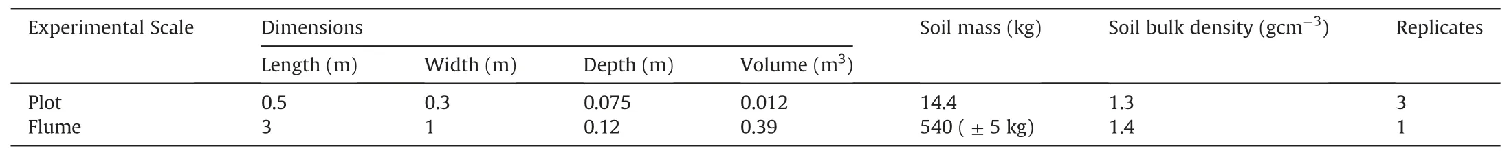
Table 1 Outline of the basic properties of the plot and flume design, where dimensions represents the volume filled with soil.

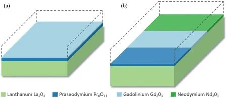
Fig.1.Schematic diagram illustrating the REO tagging design for the plots (a) and flume (b).

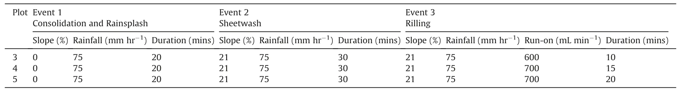
Table 2 Outline of the basic experimental conditions for each plot experiment.Rainfall intensity is correct to± 5 mm h-1 and run-on varied by± 50 mL min-1

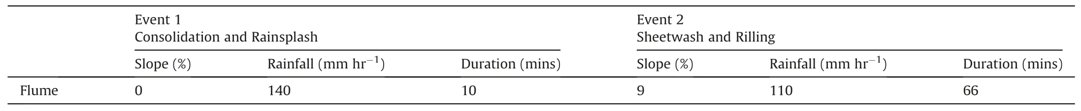
Table 3 Outline of the basic experimental conditions for the flume experiments, where rainfall intensity is ± 25 mm h-1

Li=Lt(Cmi-Cbi)/(Cai-Cbi) (1)

Equation(1):Proportional method for calculating soil loss from tagged section.

Where Liis the soil loss from the area with ith tracer(g),Ltis the total soil loss (g), Cmiis the measured tracer concentration in the sediment yield (ppm), Cbiis the background concentration (ppm),and Caiis the REO application concentration (ppm).

2.4.SfM photogrammetry

Three Canon 600D digital SLR cameras,with Canon EF-S 18-55 III lenses, were used for the plot and flume scale experiments(Fig.2).The focus and zoom were taped in place with electrical tape to mitigate any avoidable changes to the intrinsic lens geometry during the experiments.Shutter speed was set to auto and the remaining camera operative settings were kept consistent between the plot and flume scale experiments.ISO was set to 200,aperture was F8.0,exposure was adjusted to-2/3 and the highest resolution JPEG format(18 MP)was selected.Focal length was set to 21 mm for the plot experiments and 18 mm for the flume experiment.

Fig.3 provides a simple overview of the workflow that was followed for processing the above-described imagery using Agisoft Photoscan Professional version 1.2.6 (referred to herein as Photoscan).Processing was broken into two distinct stages: camera calibration and dense point cloud construction.Calibrating lens parameters prior to the collection and processing of experimental imagery reduces the need for multiple images, of varied extrinsic geometry (Eltner et al., 2017; James & Robson, 2014; Shahbazi,Sohn, Thˊeau, & Menard, 2015).As a result, the geometry of experimental imagery only needs to provide coverage of the area of interest, from a minimum of two viewpoints, similar to traditional photogrammetric studies.This allows for the use of a fixed imaging station, increasing the replicability of the overall workflow, and could permit the collection of time-lapse imagery in future applications.

Due to the scale and location of the experiments, a georeferenced coordinate system was not required, so local coordinate systems were defined using control point markers.For the plotscale work, this was achieved through the use of a ‘control frame’, which consisted of a three-tiered frame of rigid steel, with 18 markers affixed to each layer of the frame(54 markers in total).For the flume-scale work, markers were affixed to 3 sides of the flume approximately 0.12 m apart, totalling 59 markers.To allow for automated detection of control points within images, 12-bit coded markers, generated by Photoscan, were used.When defining the 3D marker coordinates, the frame tiers defined the horizonal plane,with one frame side defining the X-axis.The frame was assumed to be orthogonal and marker Z-coordinates were determined by measuring marker pair separation distances between tiers.The horizontal distance between all markers was measured with Digital Vernier Calipers (Silverline - 380244,accuracy ± 0.01 mm).

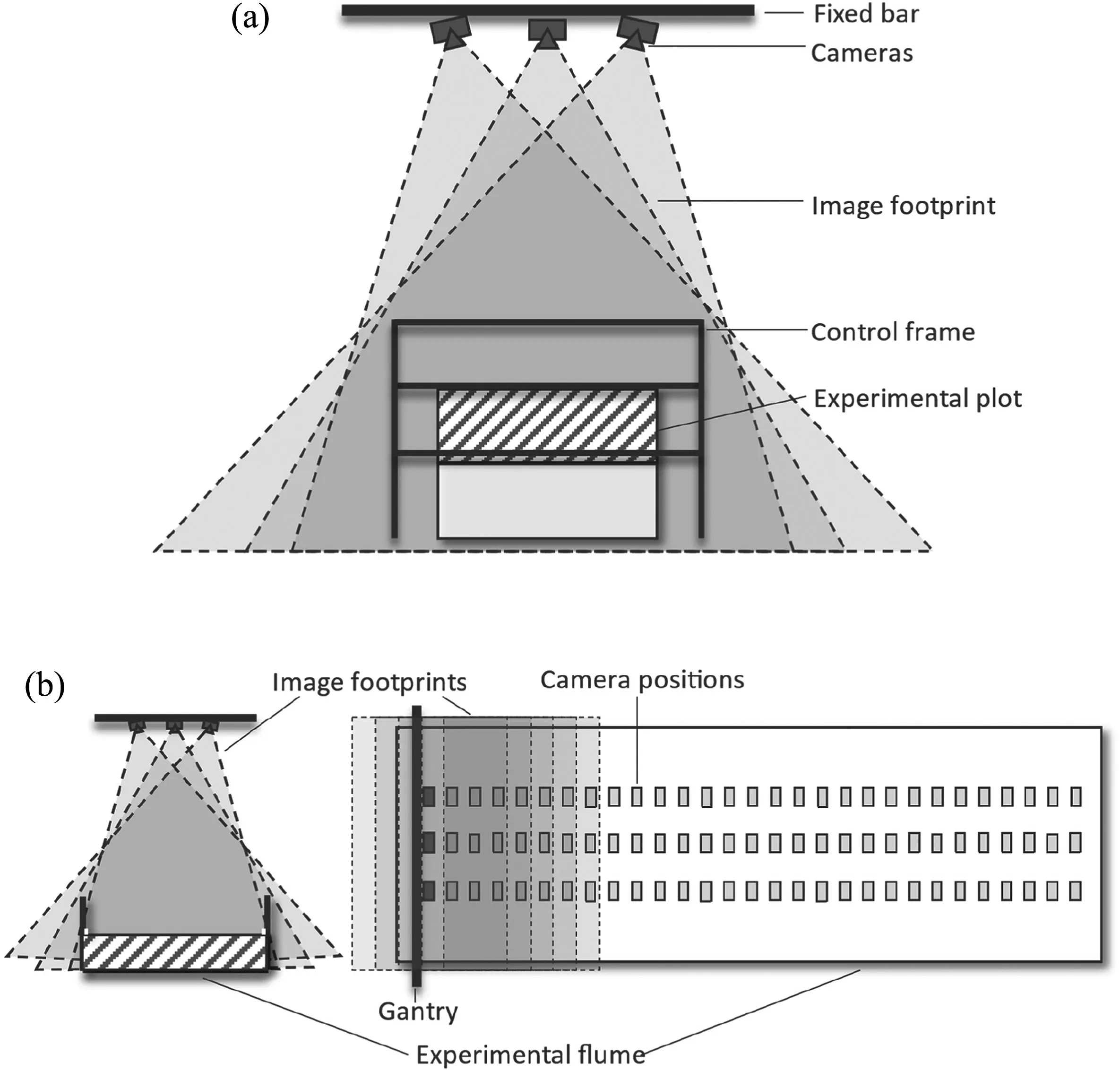
Fig.2.Schematic diagram showing the set-up used to collect experimental imagery for the (a) plot scale experiments, and (b) flume scale experiments.

As convergent imagery from each camera is particularly important for the calibration of principle point (cx and cy lens parameters; Nouwakpo et al., 2014), ca.30 convergent images of the control frame were collected with each camera, prior to running each group of events, i.e.once for each plot and once for the flume experiments.For each iteration, the calibration images from each camera were loaded into Photoscan as a single ‘chunk’,and the images from each of the three cameras were placed into three separate camera calibration groups.Following alignment,any obviously erroneous points were removed, the markers detected and defined by python script, then ‘optimisation’ or bundle adjustment was carried out using the following internal orientation parameters:cx,cy,k1,k2,k3,b1,b2,p1 and p2.The values‘marker accuracy (m)’, ‘scale bar accuracy (m)’, ‘marker accuracy (pix)’ and‘tie point accuracy (pix)’ were adjusted to match the reported values for the ‘pix’ fields and 0.5 mm for the ‘m’ fields.The calibration file for each camera and the estimated coordinates for each marker on the control frame were then exported for use in the SfM processing.

Imagery of the soil surfaces were collected immediately before and 1 h after each experimental run, for both the plot and flume scale experiments.Three cameras were mounted 0.18 m apart on a rigid aluminium bar.The central camera was nadir to the soil surface, and the outer cameras were angled at 13°for the plot scale work and 10°for the flume, to minimise systematic error effects(Heng, Chandler, & Armstrong, 2010; Wackrow & Chandler, 2008,2011), and creating 100% overlap within the area of interest between all cameras.For the plot scale experiments, an imaging station was built, as illustrated in Fig.2A.Each plot was carefully positioned within the control frame between experimental runs,where the cameras were situated 87 cm above the soil surface,resulting in a ground sampling distance (GSD) of 0.175 mm per pixel.At the flume scale,the camera bar was mounted 90 cm above the soil surface on a gantry that ran the length of the flume(Fig.2B).The bar gantry was then moved down the flume on the gantry,collecting imagery from all three cameras at 10 cm intervals,creating ca.86% forward overlap between sequential pairs.A total of 81 images were collected for every surface reconstruction (27 images per camera) with a mean GSD of 0.21 mm per pixel.

The experimental images for each surface were loaded into Photoscan and grouped according to camera.The camera calibration for each camera was then imported.The 12-bit markers were auto-detected in each image prior to camera alignment and tie point matching.Obviously erroneous points were then removed from the sparse cloud.For the plot scale experiments, the 54 marker coordinates then loaded and assigned an accuracy of 1 mm.For the flume scale experiments, the scalebar distances between every pair of markers were imported using a python script, which were assigned an accuracy value of 0.5 mm.Any markers or scalebars that appeared in only 1 image were removed.To provide a consistent assessment of model accuracy, at the plot scale, all markers present in ≤2 images were used as a check point(12-15),while at the flume scale 15%of the total number of scalebars were used as checks.Bundle adjustment was then carried out using the following internal orientation parameters:cx,cy,k1,k2,k3,b1,b2,p1 and p2, as this was found to improve model precision.Dense clouds were built using mild depth filtering and the ‘ultra-high’quality setting for the plot experiments and the ‘high’ quality setting for the flume experiments.The dense clouds were then exported as an ASCII text file.Further analysis was carried out to understand the precision and replicability of the SfM methodology,as described in Supplementary Material.

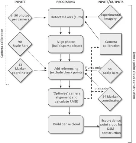
Fig.3.Workflow for the production of georeferenced dense point clouds using Photoscan.Dashed lines indicate the calibration phase, while solid lines the processing for dense point clouds.

2.5.Change detection

The final point clouds for both the plot and flume experiments were loaded into CloudCompare version 2.61 (http://www.danielgm.net/cc/) for cropping and co-registration.6 pairs of stable, matching points were selected to align each point cloud with the point cloud from time-step 1 for each experiment.Following co-registration the point clouds were trimmed to the perimeter of the soil surface to avoid including artefacts in the calculations.All temporal iterations of each plot or flume were then trimmed simultaneously, to eliminate discrepancies in the final cloud size and shape.To match the extent of REO tagging within the flume,the point cloud was then segmented into 1 m sections along the flume in CloudCompare, so volumetric estimations could be calculated for each section independently.

The co-registered point cloud data were then interpolated into Digital Elevation Models (DEMs), using the ‘gridding’ function within Surfer (Golden Software LLC, version 13.5).Kriging was selected as the method for interpolation, which the software implements with a combination of weighted averaging(i.e.the point closest to the grid node has more weight in determining the z value)and exact interpolation,when the grid point hits a raw data point, using a linear variogram.

To ensure DEM of difference (DoD) calculations only detected significant elevation changes, sources of error were combined to determine a cell-by-cell minimum ‘level of detection’ (LoD),consistent with the approach of (Smith & Vericat, 2015) following the work of (Brasington, Langham, & Rumsby, 2003; Lane,Westaway, & Murray Hicks, 2003; Wheaton, Brasington, Darby, &Sear, 2010).Three potential sources of error were identified for the volumetric calculations: SfM precision, the interpolation into DEMs and the co-registration of pairs of point clouds.The LoD was calculated for each DoD using Equation(2),which builds on the LoD equation presented by Lane et al.(2003):

Equation (2): Level of Detection for volumetric estimations between soil surface iterations.

Where,LoDiis the LoD for the ith grid cell,t is the critical t value for the given confidence interval and ε is the error associated with each metric, DEM error is the standard deviation of elevation (σz)for the ith grid cell in each DEM,i.e.DEM1and DEM2,P1and P2is the point cloud precision based on the check point RMSE values and REG is co-registration error from point cloud alignment.In this instance, a confidence interval of 95% was used (t = 1.96), and the LoD was applied as a threshold minimum level of detection.The trapezoidal rule(Fawzy,2015)method within“Surfer”was used to determine areas of positive(cut)and negative(fill)change,and the predicted volume of soil loss for each event was assumed to be the difference between the two.

The plot-scale DoDs were used to identify the total volume of change from each different REO tagged layers i.e.0 - 5 mm,5-15 mm, and >15 mm.For comparison with the REO-based calculations,volumes were then converted to a mass of soil loss using the bulk density of the initial soil mass i.e.1.3 g cm-3for the plots and 1.4 g cm-3for the flume.

3.Results

3.1.Runoff and sediment

During the plot sheetwash events(E2),runoff and sediment flux reached a steady state after approximately 10 min, across all plots(Supplementary Material,Fig.3).The maximum discharge rate was 0.0023 L s-1on P4 after 20 min, and the greatest sediment concentration was 11.97 g L-1, which was also on P4, 30 min into the event.P3 and P5 experienced a decline in sediment concentration from the 20th minute of the event.Conversely, whilst discharge reached a steady state after 2 min for all plots during the rilling experiment (E3), sediment concentration did not reach a steady state (Supplementary Material, Fig.4).With the exception of P3,sediment concentrations declined after 5 min.The inclusion of a concentrated run-on source increased runoff by an order of magnitude, accordingly, the maximum discharge rate was 0.013 L s-1,which was after 15 min on P4,and the highest sediment concentration was 109.6 g L-1on P4,6 min after the event began.

Total sediment yields and the equivalent soil volume for the experiments are presented in Supplementary Material, Table 2.At the plot scale,total sediment yield ranged between 22.5 and 31.3 g for E2,and 274.58 and 589.2 g for E3.For the E2 events,the largest calculated change was 24.1 cm3,for P4,which when averaged over the area of the plot equates to a mean denudation of 0.016 cm.There was no visual evidence of rilling or nick-point formation during all plot scale E2 experiments, consistent with sheetwash erosion being the dominant erosion process.For the E3 events,this equated to a calculated maximum volume change of 453.2 cm3on P5 and a minimum change of 211.2 cm3for P3, with total change increasing with event duration.In all instances, the addition of a runoff source(E3)led to the formation of a rill feature and soil loss an order of magnitude greater than E2.

The PSD of the original soil and was compared with the PSD of the exported sediment(Fig.4-plots;Fig.5C-flume).At the plot scale, there was a significant difference between the PSD of the bulked sediment from E2 and E3,for all classes bar the silt and clay fraction(<63 μm)(ANOVA,F(1,6)=6.891,p=0.039).Furthermore,there was a preferential transportation of the medium to fine sand particles (500 > 125 μm) and the silt and clay fraction (<63 μm)during the sheetwash experiment (E2).In contrast, for the rilling experiment (E3) there was only evidence of preferential transport of the silt and clay fraction.Across all events,the fine gravel fraction(>2000 μm)was under-represented within the exported sediment.The export of both the fine gravel and very coarse sand fraction(>2000 and 2000 > 1000 μm) did, however, increase with event magnitude.

During the flume sheetwash and rilling experiment, an approximate steady state of runoff was reached after 34 min(Fig.5a).There was however an on-going slight increase in discharge from this point, ranging from 0.094 L s-1at 34 min to 0.096 L s-1at 66 min.An approximate steady state of sediment concentration was reached after 16 min.The mean steady state sediment concentration was 11.4 g L-1(±1.02).There was a final peak in sediment export at minute 58, where sediment concentration was 14.4 g L-1,as visible in Fig.5b.The total sediment yield for the experiment was 3914.1 g.

Analysis of the PSD of the exported sediment (plotted as enrichment ratios,relative to the original soil,Fig.5c)show that the fine gravel fraction (>2000 μm) and the coarse sand fraction(2000 > 1000 μm) were under-represented in the sediment exported from the flume.There was evidence of the preferential transport of the fractions finer than 1000 μm,most notably the silt and clay fraction(<63 μm),which had an enrichment ratio of 3.4 in the bulked analysis.The concentration of the<63 μm fraction was the greatest in the initial sediment sample, representing an enrichment of 12.2 (not visible in Fig.5c due to scaling).The 500 > 250 μm and 250 > 125 μm fractions, the fine and medium sands, were the most eroded, representing 27.6% and 23.4% of the total exported sediment,respectively.Whilst this is also consistent with the PSD of the original soil, both fractions had a cumulative enrichment ratio of 1.2.

3.2.REO tracers

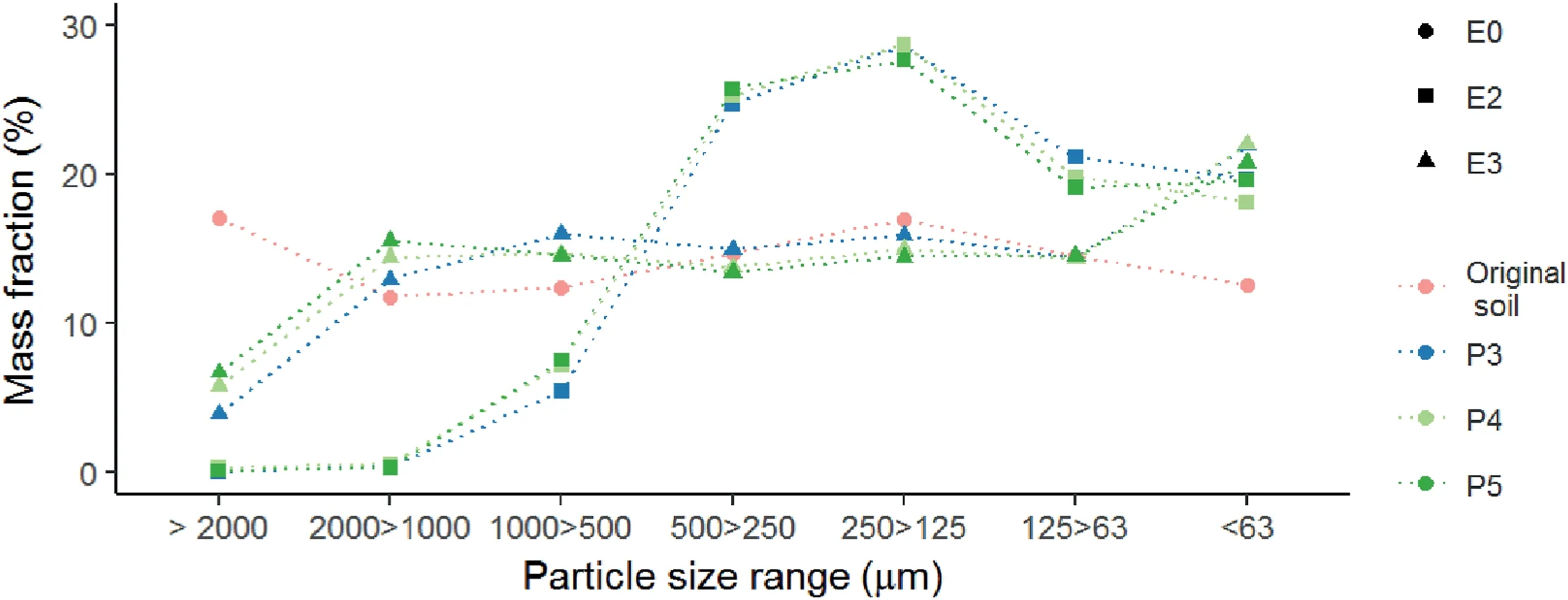
Fig.4.PSD for bulked sediment samples following experimental runs two and three, presented as mass faction (%) for each φ interval.Where E0/pink is the original soil, E2 is sediment exported during the sheetwash experiment, and E3 is sediment exported during the rilling experiment.

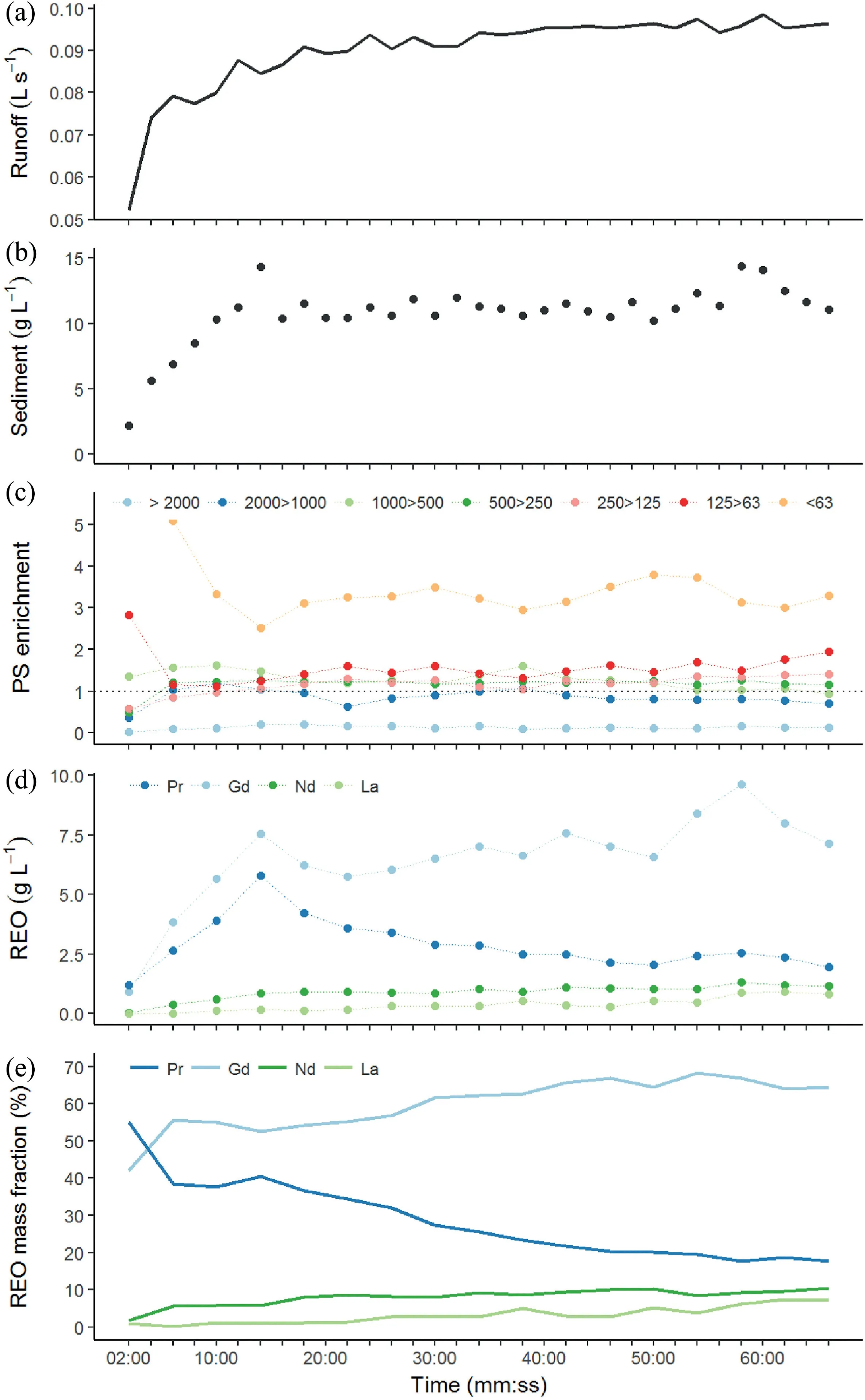
Fig.5.Summary of flume discharge(a),sediment concentration(b),enrichment of particle size fractions(c), REO-based concentrations calculated from the sediment samples(d),and REO-based sediment apportionment (e), through time during Event 2.

The REO-derived calculations indicate that the top 5 mm of soil within the plots was the primary source of sediment during the sheetwash experiment(E2),accounting for over 99%of all soil loss,as visible in Fig.6a.The mass of soil exported from the top layer of soil ranged from a minimum of 20.04 g on P3,to a maximum of 28.26 g on P4.During E2,a maximum of 0.28 g of soil was exported from the second soil layer(5-15 mm),which was on P4.Based on the relative REO concentrations, the top 5 mm of the soil profile was also the main source of sediment during the rilling experiments (E3), as shown in Fig.6b.Soil loss from the top layer ranged from a minimum of 114.0 g on P3 to a maximum of 228.9 g on P5, accounting for between 39.1 and 41.5%of the total sediment yield.The middle layer contributed 30.6-40.4%of the total sediment yield.Accordingly,soil from the depths greater than 15 mm contributed the least to the total sediment yield.The relative contribution from depths >15 mm increased with event magnitude and ranged from a minimum of 18%on P3 to a maximum of 29.4%on P5.

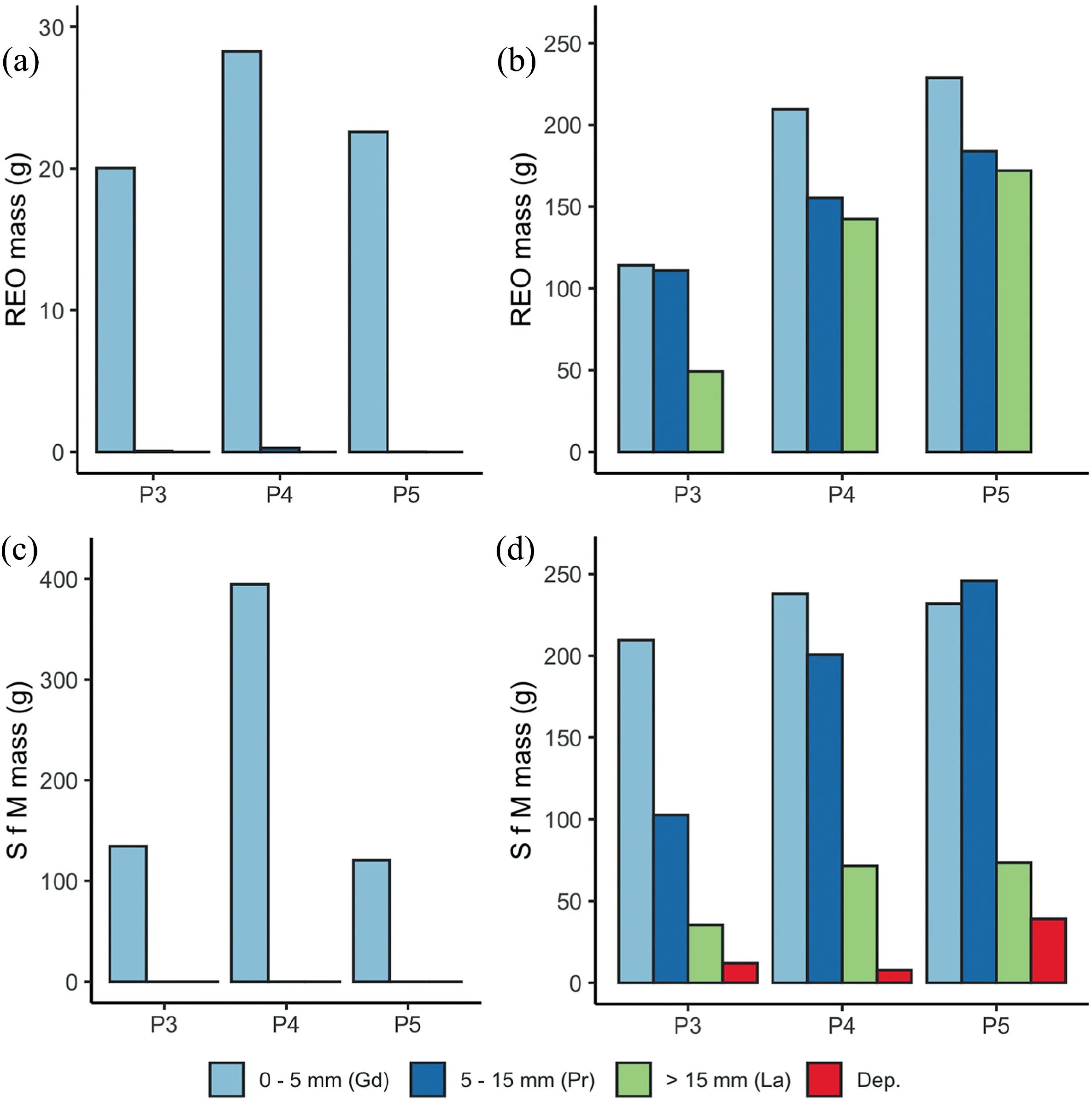
Fig.6.Calculated contribution from each tagged layer in the plot soil profile based on REO concentrations in the bulked sediment samples for(a)the sheetwash events(E2),and(b)the rilling event(E3).Calculated contribution from each tagged layer in the soil profile based on SfM-derived elevation and volumetric change for(c)event 2,and(d)event 3,where‘Dep.’ represents the positive change resulting from sediment deposition.Note the different y-axis scales.

In the flume experiment,the REO concentrations in the sediment samples indicated that the Gd-tagged portion of the soil, the upper 10 mm of soil profile 1-2 m from the top,was the greatest source of exported sediment, as shown in Fig.9a.Based on the REO-based calculations, a total of 2395.5 g of soil was exported from this section (61.2%), in contrast with 1038.3 g (26.5%) from the Pr-tagged section (2-3 m from the top of the plot, closest to the exit) and 334.3 g(8.5%)from the Nd-tagged section(0-1 m from the top of the plot).The maximum concentration of sediment from any one section was 9.6 g L-1, which was from the Gd-tagged section (Fig.5d).The relative contribution of sediment from the Gd-tagged zone increased throughout the experiment(Fig.5e).Similarly,the relative amount of soil from the Nd and La sections increased throughout the experiment.The Nd section contributed 5%of the sediment flux in the 4th minute, increasing to a maximum 10% at the 66th minute.Conversely,the contribution of sediment from the Pr section,whilst greater than that from the Nd section overall,decreased throughout the experiment.There were two slight spikes in La contribution,which were 38 and 50 min into the erosion event,and 5.1 and 5.3%of the sediment flux, respectively.The La-tagged soil apportionment increased to a maximum of 7.5% of sediment flux, and contributed 3.6%(140.5 g)of the total sediment yield.

3.3.SfM photogrammetry

The mean point density of the plot SfM clouds was 3496 points per cm2and the mean GSD was 0.17 mm/pixel (Supplementary Material,Table 3).The RMSE for both the control and check points for the plot and flume experiments are presented in Table 4.RMSE values ranged from 0.16 to 0.43 mm for the plot check points.At the flume scale,the mean point density was 803 points per cm2and the mean GSD was 0.21 mm/pixel.The RMSE values for the check scalebars used in the flume experiments ranged between 0.15 and 0.27 mm.0.5 mm resolution and 5 mm resolution DoDs were created for each event, for the plots and flumes, respectively.

At the plot scale, the maximum negative elevation changes resolved by the SfM DoDs for ‘consolidation and rainsplash’ (E1)and ‘sheetwash’ (E2) experiments ranged from -3.6 to -5.5 mmand -3.9 to -7.2 mm, respectively, based on the 0.5 mm DoDs shown in Fig.7.The minimum rill depth was 32.2 mm,for P5.There were areas of positive surface elevation change also detected for all plots following E3.These ranged from a minimum increase of 5 mm on P3 to a maximum of 9.2 mm on P5.The most significant areas of positive elevation change resulted from areas of sediment deposition from the primary rilling feature (Fig.7).

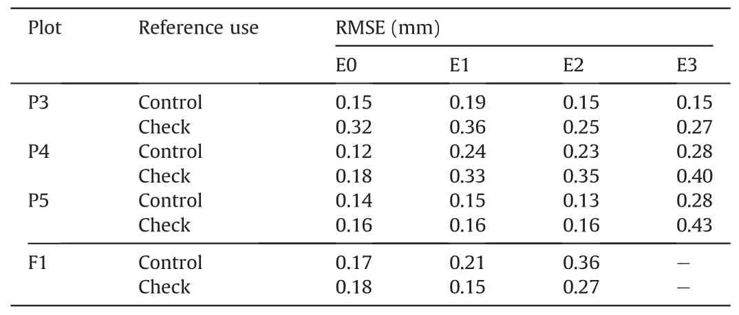
Table 4 RMSE values of the control and check points for each plot SfM-MVS point cloud.Where E0 is the SfM model of the soil surface prior to the consolidation and rainsplash experiment (E1), E2 is after the sheetwash experiment and E3 the rilling experiment.

The SfM derived point clouds and DoD could be used to visually identify patterns and changes in the surface structure following the different events(Figs.7 and 8).Smaller depositional features,such as a secondary area of deposition located 0.2 m from the top of P5-E3,associated with a depositional area from earlier in the evolution of the central rill, could be identified using the 0.5 mm DoDs as visible in Fig.7.The elevation changes predicted for the sheetwash and rilling experiments could be used to resolve the features visible in the raw imagery.This included the lowering of the soil surface around aggregates during E2 and the presence of large aggregates in the bottom of the rill.Similarly, the flume DoD captured the features visually identified within the soil surface, including the formation of small rills up to 15 mm in depth and the deposition feature at the exit of the flume,showing accumulations of soil up to 15 mm high, while large aggregates are clearly visible in the point cloud (Fig.8a).

At the plot scale,the SfM-derived calculations show that the top 5 mm of the soil was the primary source of soil loss during E2,accounting for over 99.9% of the total changes identified (Fig.6c).Based on the SfM models, the magnitude of soil loss from the top 5 mm of the soil profile ranged from a minimum of 120.4 g on P5 to a maximum of 394.8 g on P4.The SfM DoD found that elevation changes did exceed 5 mm on P4,however,these only equated to a soil mass of 0.02 g, or a 0.005% of the total(Fig.7).

The SfM DoD indicates that soil was eroded from all three layers of the soil profile, across all plots, during the rilling experiments(E3),as visible in Fig.6d.The volumetric predictions show that the top 5 mm of the soil profile was the also greatest source of sediment during E3, for P3 and P4, contributing 60.3 and 46.6% to the total sediment yield,respectively.Conversely,for P5,the 5-15 mm layer had the greatest soil loss, accounting for 44.6% or 245.7 g of the total.The SfM DoDs show that the magnitude of soil loss from depths greater than 15 mm increased with event duration.Accordingly,the calculated mass from this section was the greatest for P5, equating to 73.4 g and 13.3% of the total.The mass of soil transported but deposited in a fan within the plot(calculated from net positive elevation changes)ranged from 39.0 g on P5 to 7.8 g on P4, and was therefore not related to event duration.

Supplementary Material Fig.5 demonstrates the spatial extent of elevation changes within the three layers presented in Fig.6,following E3, for P3 and P5 for contrast.The spatial extent of the elevation changes indicates that the rilling feature was the greatest source of sediment material during E3.Negative elevation changes covered 79%of the surface of P3 and 64%of P4,and were not limited to the rill.Negative elevation changes covered 41%of the surface of P5, and were primarily limited to the rill.All elevation changes 5-15 mm into the soil profile were confined to the rill.Elevation changes greater than 15 mm were limited to the top half of the plot length.

Fig.9 presents the predicted mass of soil lost from each section in the flume,based on the REO concentrations(Fig.9a)and the SfM DoDs(Fig.9b).Based on the total negative elevation changes within the different tagged sections, the SfM DoD found that the Gdtagged portion experienced the greatest soil loss, representing 58.7% of the total.The Nd-tagged section represented 12.9% of the total negative changes and the Pr-tagged area, closest to the exit,represented 28.3%.Accordingly,the SfM-derived calculations of soil loss from each section were strongly correlated with the REOderived estimations of apportionment (R2= 0.981).However, as shown in Fig.9,the SfM DoDs overestimated the total mass of soil loss from each section,except the La tagged layer,where soil losses were underestimated(Table 2,Supplementary Material).The areas identified within the SfM DoD as having negative elevations changes greater than 10 mm were consistent with visual observations during and after the experiment,which are coloured green inoverestimated for both P4 and P5, by 29.3 and 33.6%, respectively.The total relative measurement error of the SfM approach for the plot scale experiments, taking into consideration the mass of soil deposited,ranged between-0.95 and 22.4%.For the flume results,when compared to the REO calculations, the SfM-based calculations overestimated soil loss from the top 10 mm of the soil profile,with the greatest overestimation in the section of the flume furthest from the exit(Nd),while underestimating soil losses from the>10 mm tagged depth(La).Taking into consideration the mass of soil deposited,this resulted in a total relative measurement error by SfM of 41.9%.

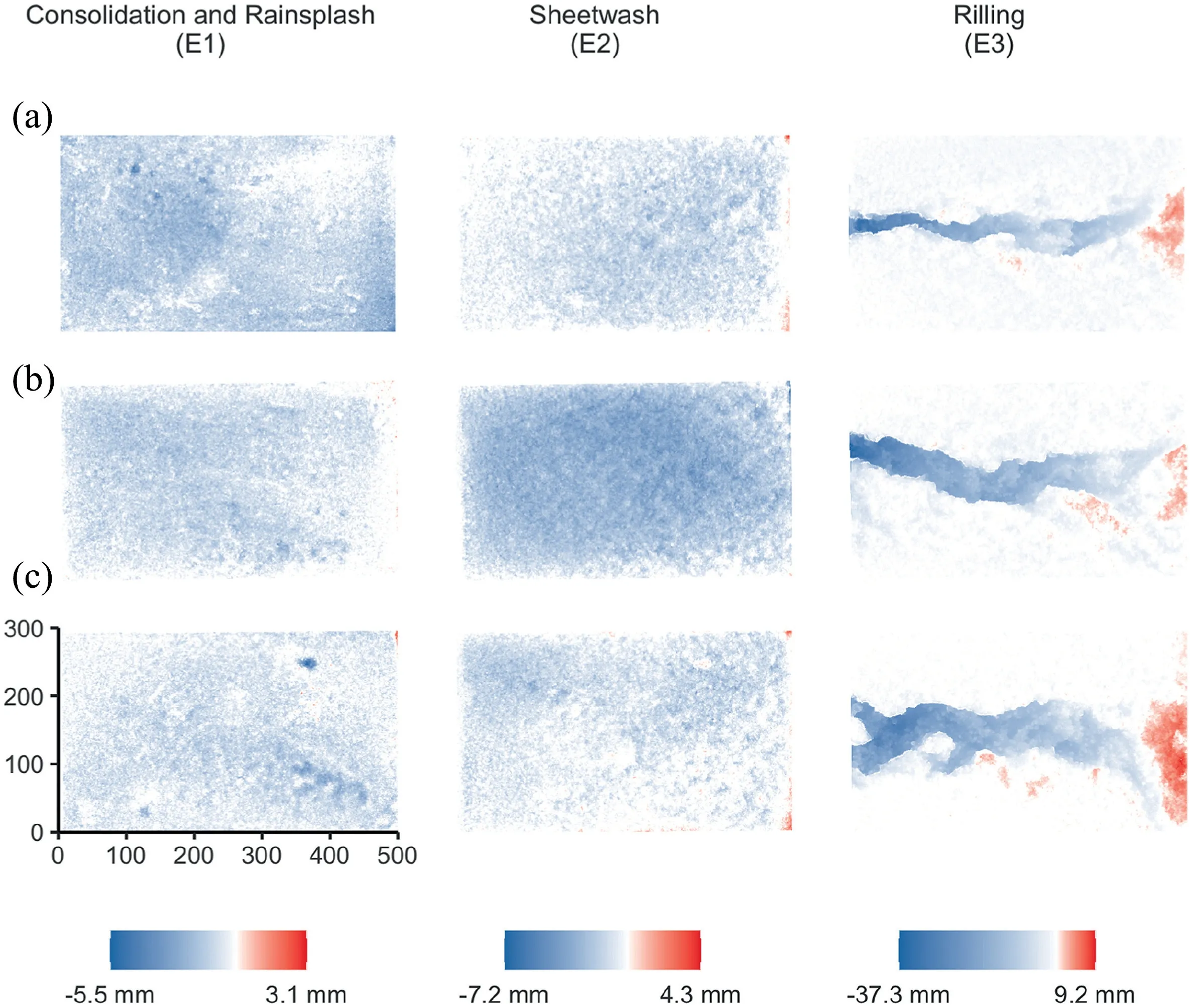
Fig.7.0.5 mm resolution DoD showing changes in surface elevation following E1,E2 and E3,for Plot 3(a),Plot 4(b),and Plot 5(c).Where,all units are mm,white represents areas with zero elevation change, blue indicates areas of elevation decreases and red areas of increased surface elevation, and flow direction is left to right.

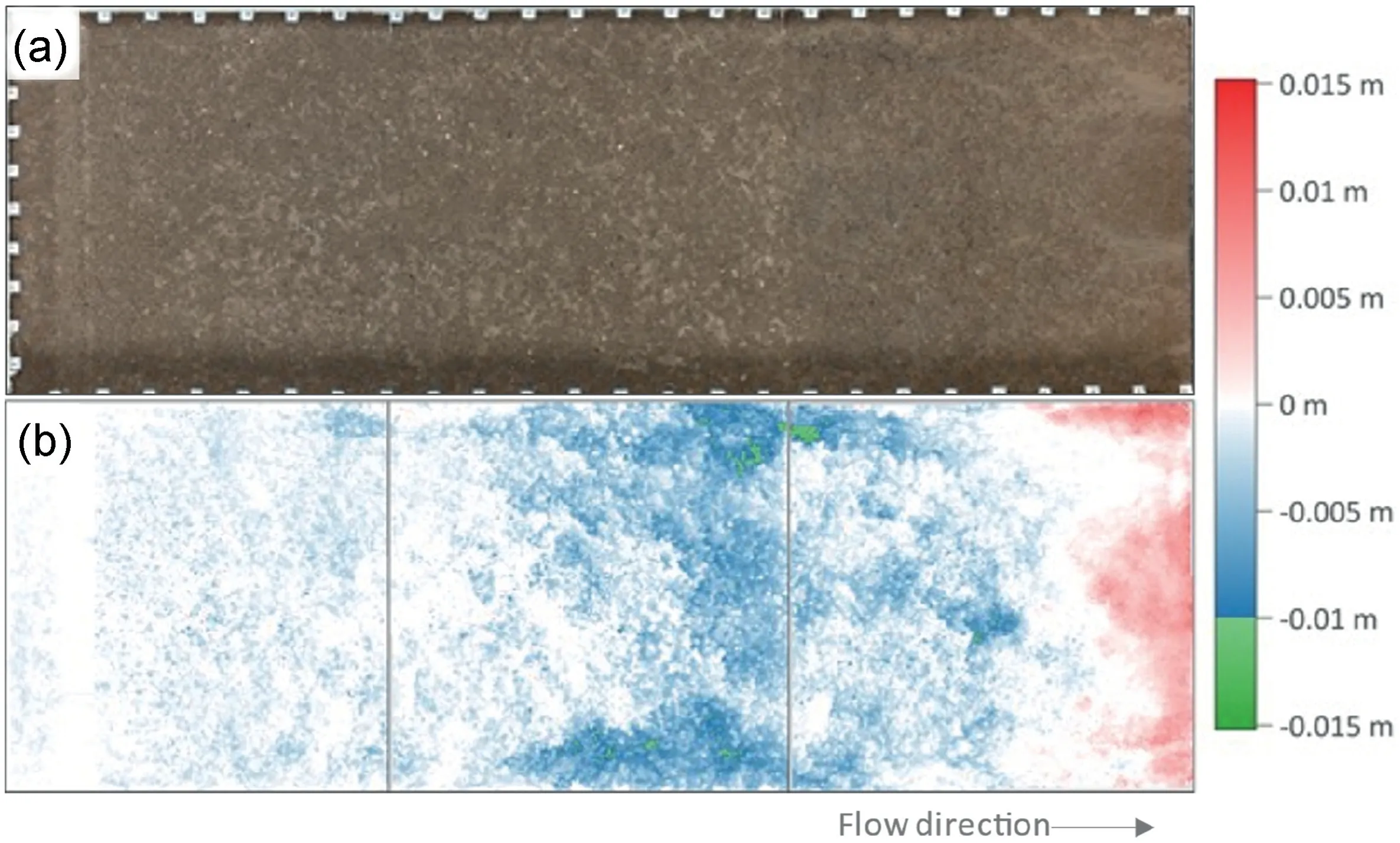
Fig.8.SfM point cloud showing the surface of the flume following the erosion experiment(a),and the associated DoD,illustrating the spatial distribution of elevation changes(b),where the DoD is coloured green in areas where the depth of soil loss exceeded 10 mm,for visual comparison with the REO tagging,blue areas of soil loss and red indicating areas of increased surface elevation.

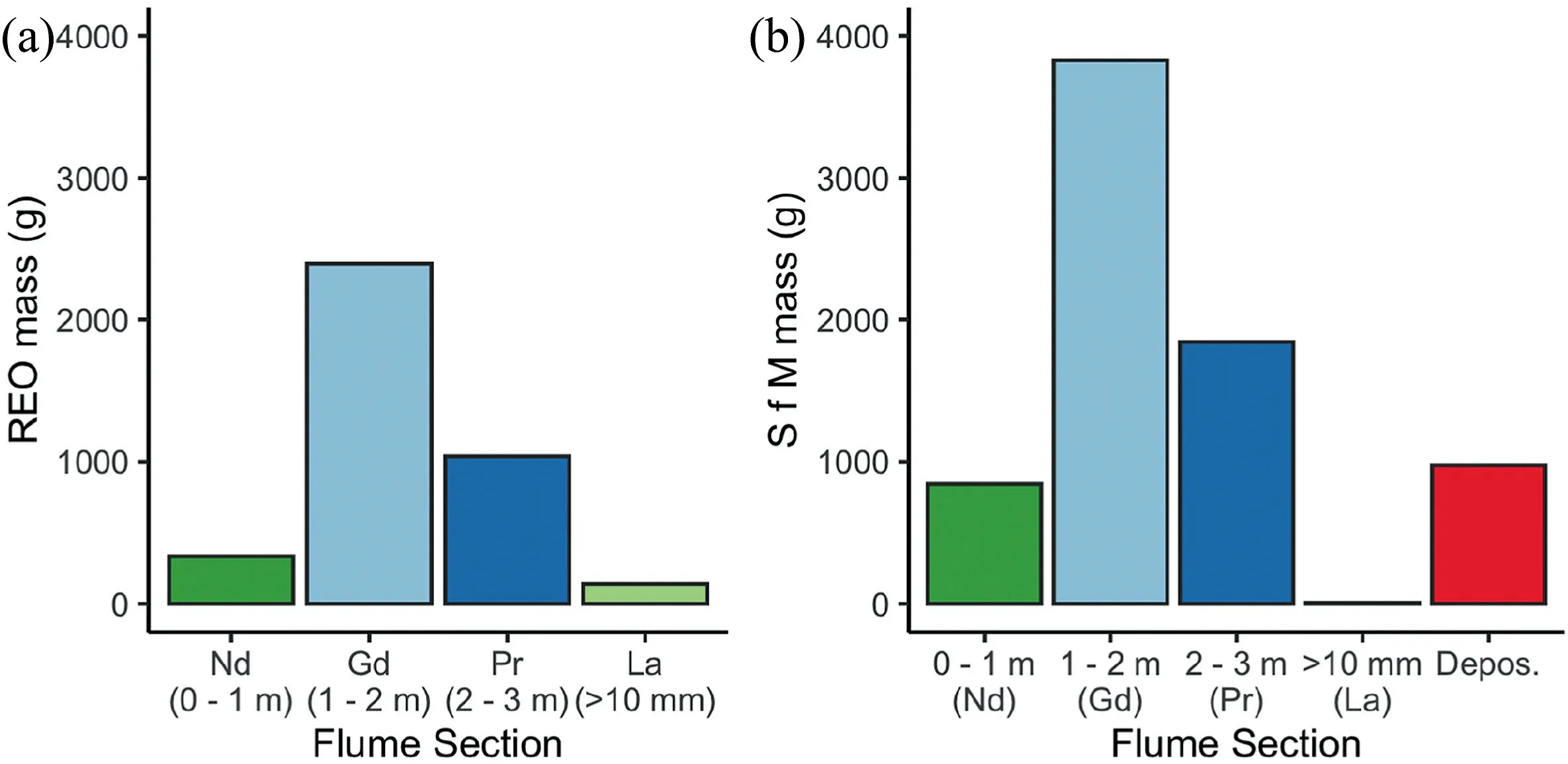
Fig.9.Calculated contribution from each section in the flume based on REO concentrations in the bulked sediment samples(a)and SfM volumetric changes within each section(b),where ‘Depos.’ indicates the mass calculated from positive elevation changes at the lower end of the flume.

Fig.8.The mass of soil transported but deposited in the Pr-tagged section of the flume, based on positive elevation changes, was 975.4 g.
The predicted soil loss resulting from the plot scale sheetwash were overestimated by SfM, ranging from a 377-1850% overestimation of soil loss.Following E3, the SfM approach overestimated the mass of soil loss from the top 5 mm on all plots,ranging from maximum of 83.8%on P3,to a minimum of 1.3%on P5,relative to REO (Fig.10).Similarly, in all instances the SfM calculations underestimated the mass of soil exported from depths greater than 15 mm (the La tagged section), ranging from a minimum of -28.2% on P3 to a maximum of -57.3% on P5.Conversely, the relative error of the predicted mass of soil loss between 5 and 15 mm into the soil profile was underestimated by-7.6%for P3,and

4.Discussion

4.1.Can sediment capture and REO tracers describe soil erosion processes under diffuse and convergent experimental conditions?

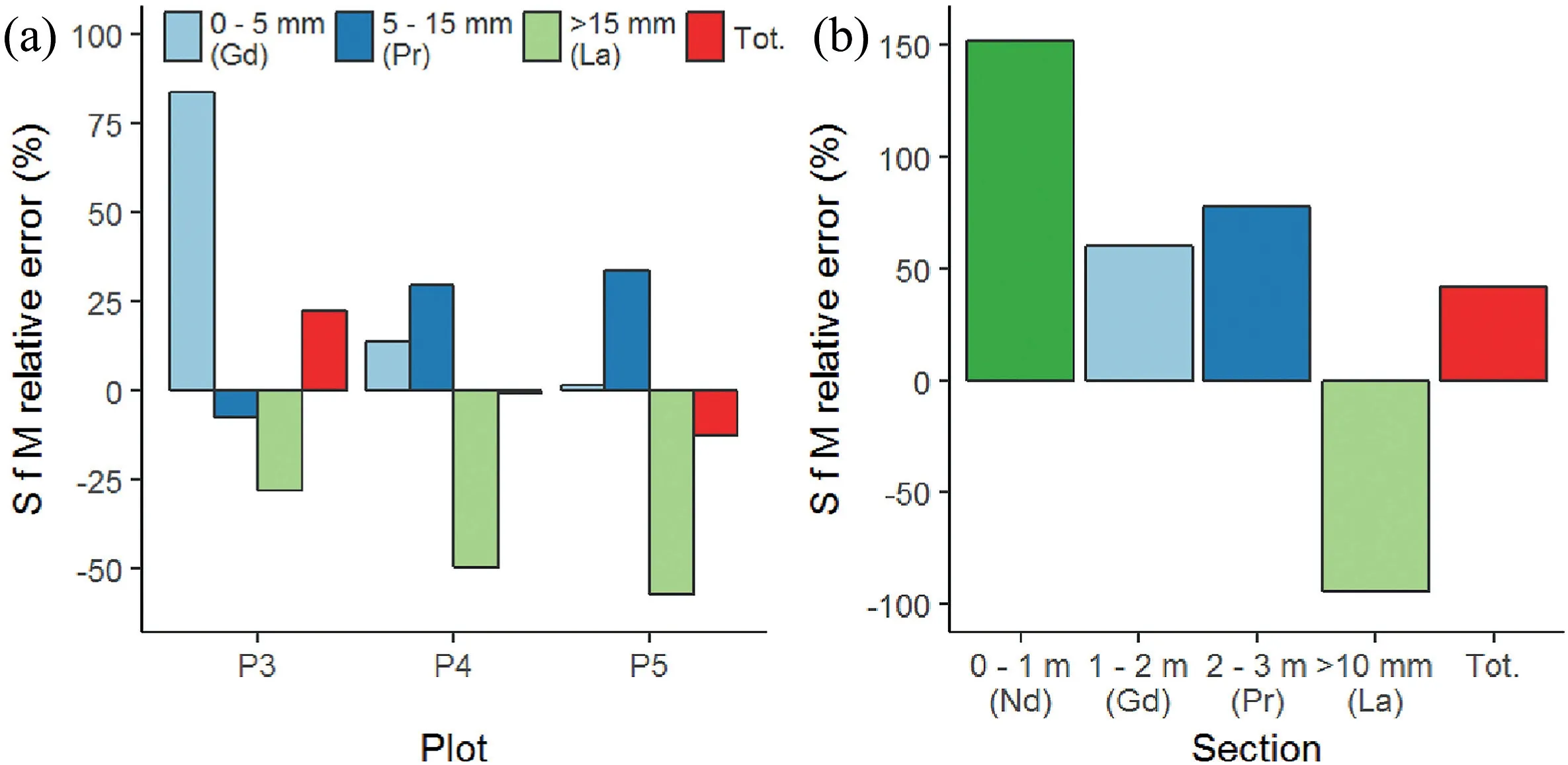
Fig.10.The relationship between mass calculated by REO and SfM,presented as the relative error of the SfM predictions when compared to the REO results.Tot.indicates the total measurement error, including the estimated mass of deposited sediment.

Experimental observations suggest that the consolidation and rainsplash events (E1) resulted in a lowering of the soil surface,consistent with the breakdown of aggregates and the lowering of the soil surface due to consolidation (Ghadiri & Payne, 1977;Kinnell,2005;R¨omkens,Helming,&Prasad,2002).The sheetwash erosion experiment on the plots (E2) resulted in the preferential transport of fine sediment(<500 μm)across all three plots(Fig.4),consistent with the sheetwash erosion described by (Armstrong et al., 2011).Discharge and sediment concentration reached a steady state across all plots, however the decline in sediment concentration following 20 min of runoff on P3 and P5 suggests that there was a depletion of readily available material during the final third of the experiments.While this could have been caused by an exhaustion of the finer sediment fractions,sealing of the soil surface by particles dispersed by the slaking of aggregates presents a more likely explanation (Le Bissonnais et al., 2005), as a smoothing between the remaining aggregates was visible on the soil surface.Conversely, following a temporary decline, sediment concentrations increased towards the end of E2 on P4.The REO concentrations indicate sediment was only sourced from the top 5 mm of the soil profile for P3 and P5, while there was some transportation of sediment from depths greater than 5 mm on P4.As the top layer of the soil had an initial air-dried mass of 900 g(versus 31.3 g of exported sediment),this suggests that the ingress into the second layer was due to a breach in the surface seal caused by increased sheer stress, rather than the exhaustion of the top layer of the soil profile (Morgan,1995).

The introduction of a single run-on source for E3 (the rilling experiment) lead to the formation of a rill on all three plots.Changing the hydrological event duration and magnitude resulted in rills of varied spatial extent, and was thus ideal for testing the application of the techniques on laboratory-scale convergent soil erosion features.Consistent with erosion from convergent features,there was less evidence of size selectivity in the sediment (Fig.4)(Alberts et al., 1980).Coarse-grain sediment (>2000 μm) was,however,under-represented relative to the PSD of the original soil.Accordingly, large aggregates (>2000 μm) were visible in the bottom of the rills on all plots.With the exception of P3, which was subjected to the smallest hydrological event, sediment concentrations declined after 5 min, indicating that following the cutting of the rills, the systems were detachment limited (supplementary material, Fig.4).Despite this, the sediment PSD and aggregates deposited within the rill shows that there was insufficient erosive energy within the system to carry the larger aggregates out of the plot.The REO tracer concentrations in the exported sediment show that the top 5 mm of the soil profile was a significant source of sediment during E3, accounting for between 39.1 and 41.6% of exported sediment, suggesting that sheetwash was also a significant route of soil loss during the E3.Interestingly,although the two combined layers represent a greater sediment source than the top 5 mm of the soil profile, the REO tracers illustrated that the total exported mass apportioned to each individual layer was less than that of the top 5 mm,despite a greater initial resource.Of the two layers deeper than 5 mm, the REO calculations illustrated that the 5-15 mm layer was the greatest source of sediment.This indicates that transport efficiency declined as the rill matured, which is consistent with the reductions in sediment concentration (shown in Supplementary Material, Fig.4)

4.2.Do SfM photogrammetry derived volumetric changes agree with soil loss quantified by sediment capture and REO tracers?

SfM photogrammetry consistently overestimated soil loss from the sheetwash experiment,suggesting that further consolidation of the soil profile may have occurred during the sheetwash experiment, and could indicate that further saturation of the already moist soil lead to further aggregate disintegration or deformation(Bryan, 2000).This also aligns with the findings of others in both SfM and LiDAR applications (i.e.Balaguer-Puig, Marquˊes-Mateu,Lerma, & Ibˊa˜nez-Asensio, 2017; Kaiser, Erhardt, & Eltner, 2018;Polyakov&Nearing,2004),where non-soil loss related decreases in surface elevation i.e.compaction and surface consolidation, were found to mask/exceed soil loss via diffuse pathways.Assuming the difference between the volume of sediment collected and the SfM DoD estimations of volumetric change was soil structure consolidation,SfM could detect a mean bulk density increase of 0.04 g cm3.

Patterns of soil loss present within the DoDs matched visual observations during the rainfall events,and suggest that during the experiment networks of aggregates shifted downslope by the moving water, creating shallow flow paths, facilitating the development of higher velocity flows(Slattery&Bryan,1992).Consistent with this, and matching the REO results, SfM indicated that sediment was sourced from depths greater than 5 mm on P4.Interestingly, while the SfM DoDs overestimated the total mass of sediment exported via sheetwash from the plots, the mass of sediment apportioned to depths greater than 5 mm was underestimated when compared to the REO results.This suggests that there was some deposition of sediment within the feature, and indicates that there was not sufficient energy within the system for convergent flow paths to form (Slattery & Bryan,1992).

Following the rilling plot experiment,SfM found soil losses to a maximum depth of ca.2 mm covered 79%of the soil surface outside of the rill on P3 and 49%of the soil surface on P4,correlating with the suggestion that sheetwash also contributed to soil loss.The DoD indicate that all soil loss from depths greater than 5 mm were sourced from within the rills (Supplementary Material, Fig.5).However, the SfM calculations under-estimated the mass of exported sediment apportioned to depths greater than 15 mm,while over-estimating the losses between 5 and 15 mm for P4 and P5, suggesting that sediment from all layers was deposited within the rill.Conversely, for the smallest rill, P3, the SfM technique under-estimated soil losses from both layers greater than 5 mm deep, while over-estimated soil losses from the top 5 mm.The overestimation of soil losses in the top 5 mm, most likely resulted from the continued deformation of the soil surface via slaking.The under-estimation of soil loss on P5 could have resulted from an uplifting of the soil profile cause by swelling, or an inappropriate application of the LoD model to the DoD calculations.Overall,SfM had lower relative measurement errors for E3 than E2,indicating a stabilisation of the non-erosional processes, such as aggregate breakdown and compaction, within the soil profile.Promisingly,this suggests that SfM could capture diffuse soil losses should soil beds be allowed to consolidate(either naturally,or through rolling)prior to the start of the measurement period.

The RMSE of the check points was consistently higher than that of the control points for the plot experiments SfM photogrammetry,suggesting that the precision values used for the control points could have been increased to allow the photogrammetry to have a greater influence over the model construction.This is likely not uncommon, and highlights the need for reporting full GCP RMSE information for better transparency in the presentation of model quality/precision (James, Robson, D’Oleire-Oltmanns, &Niethammer, 2017; Smith & Vericat, 2015).When the RMSE values are transformed into relative precision ratios relative to survey range (James & Robson, 2012), the values gained from this experiment ranged from 1:2000 to 1:6200, and were therefore superior to ranges achieved within the field-based studies described by Smith et al.(2016).The technological advances, relative to the then very much state of the art digital photogrammetry models by Rieke-Zapp and Nearing(2005),have afforded an order of magnitude increase in DEM resolution(0.5 mm vs.3 mm)and zprecision (0.17 mm vs.1.26 mm).

The trialled precision analysis does suggest that there is scope for even further improvements in SfM point clouds precision,through better constraint of the model (James, Robson, D’Oleire-Oltmanns, & Niethammer, 2017; James, Robson, & Smith, 2017).This could be achieved through either collecting imagery with greater variations in extrinsic geometry i.e.the inclusion of greater number of camera orientations from each camera(James&Robson,2014) or a better distribution and precision of GCPs coordinates(James, Robson, D’Oleire-Oltmanns, & Niethammer, 2017).The‘shape only’ precision for the plot scale (Supplementary Material,Fig.1) suggests that while the consideration of the photogrammetric requirements was sound,the collection of more precise GCP information could have improved the ‘georeferenced’ precision(James, Robson, & Smith, 2017).However, at 0.5 mm, it could be suggested that the GCP precisions achieved were already at the limit of that practically achievable at this scale.

4.3.What is the spatial and temporal pattern of soil loss and source apportionment during soil erosion events?

Following the initial consolidation rainfall event, a single erosion experiment was carried out on the flume,which resulted in a mean surface lowering of 1.4 mm.Observations during the rainfall event indicated that sediment was transported in flows more consistent with interrill erosion than rill, although some small convergent features were visible towards the end of the experiment.Following the experiment, qualitative observations suggested that surface lowering was primarily situated around large aggregates on the soil surface, which was also visible in the SfM point cloud and DoDs (Fig.8).Unlike the plot scale sheetwash experiments, the bulked PSD of the exported sediment was not significantly different to the PSD of the original soil.However,there was a mean enrichment of 3.9 for the<63 μm fraction throughout the experiment, and sediment fractions between 500 and 125 μm represented over 50% of the total yield.This is consistent with the plot scale sheetwash experiment, however, unlike the plot experiments, sediment concentrations did not decline with time, suggesting that there was not an exhaustion of material or similar level of sealing on the soil surface.These findings correlate with the known vulnerability of sandy loam soils, as used in these experiments to sheetwash and soil erosion more generally(Benaud et al.,2020).

Analysis of REO concentrations within the exported sediment revealed that the middle section of the flume, which was tagged with Gd (1-2 m from the top) was the primary sediment source(Fig.9).This is consistent with the findings of Polyakov and Nearing(2004),who were working with a 4 m long flume.For the first timestep, however, the section of the flume nearest to the exit (tagged with Pr)was the dominant soil source,contributing 60%of the total sediment yield and the mid-section contributed 40%.While the mid-section of the flume was the primary source of exported sediment for all subsequent samples,the sediment concentrations from both the mid-section and the section nearest the exit continued to increase for the first 14 min of the experiment,matching increasing discharge.However, after steady state was reached,the amount of sediment exported from the final metre of the flume decreased for the remainder of the experiment.This also coincided with a gradual increase in sediment sourced from the section furthest from the flume exit,tagged with Nd,indicating that sediment travel distances did reach at least 2 m during the experiment.The results therefore demonstrate that as the flow pathways became more connected along the length of the flume,the carrying capacity that remained after the mid-section of the flume decreased,which suggests that some sediment was transported in suspension.

Given the dominance of sheetwash erosion during the experiment, only 3.6% of the sediment was sourced from within the Latagged mass.The patterns of soil loss identified by the DoD for negative elevation changes greater than 10 mm were, however,visually consistent with the features typical of rill initiation as found by Bryan and Poesen(1989),for example.This suggests that the flow rate of the moving water had reached critical sheer stress and, should the experiment have run for longer, suggests the rills would have continued to develop.However, while SfM overestimated soil loss from all three sections along the flume length,losses from the La-tagged soil were underestimated.This suggests that there could have been some back-filling of the rills with sediment transported from upslope,consistent with the theory that most sediment is moved downslope in a series of short movements(Kirkby,1991;Parsons et al.,1998;Wainwright et al.,2008).Indeed,the Nd-tagged section had the greatest relative error between SfM and REO calculations, identifying a potential source of the deposited sediment.However, unlike the plot scale experiments, visual inspection of the SfM DoD and point clouds illustrate that the soil surface within the convergent features was smooth, rather than covered with large aggregates, indicating that deposited material primarily consisted of disaggregated soil particles.

4.4.The future use of REO tracers and SfM photogrammetry to elucidate retrospective information on soil erosion processes

The laboratory scale experiments presented herein have afforded an opportunity to describe the relative contribution of diffuse and convergent soil erosion processes through the applying REO tracers in stratified manner in combination with SfM photogrammetry.Furthermore, the added information provided by a spatial and stratified tagging approach, along with a temporal analysis of sediment tracer composition, allowed a spatiotemporal understanding of sediment transport distances and the temporal evolution of soil erosion processes to be described.While SfM photogrammetry was able to resolve sub-millimetre changes in surface elevation, demonstrating a strong potential to quantify diffuse soil erosion pathways, non-soil loss changes to elevation such as consolidation of soil structure, compaction, swelling and aggregate breakdown,were found to be greater than rates of diffuse erosion.However, it is expected that non-erosional surface elevations changes would decrease after sequential erosion events(Polyakov&Nearing,2004),suggesting SfM photogrammetry could be used to resolve diffuse erosion losses in repeated experiments,or in field conditions where there is limited disturbance to the soil structure prior to the soil erosion observations,as demonstrated by C^andido, James, et al.(2020) and C^andido, Quinton, et al.(2020).Reducing the limit of detection for DoD calculations could also improve confidence in the SfM calculations, and allow nonerosional changes to the soil surface to help describe further processes involved in soil erosion.

The use of an imaging station and pre-calibrated camera models reduces data collection and processing times, while producing high-precision point clouds for plot scale experiments, and thus offered a replicable and robust methodology which could be applied to time-lapse acquisitions along-side sediment and tracer collection.At the field scale,a repeat of the watershed experiment by (Polyakov et al., 2009) with the addition of droned-based high resolution SfM photogrammetry could substantially reduce the amount of coring needed, while increasing the spatial understanding of soil redistribution and loss, despite the partial tagging of the soil profile.In fact, changes in the enrichment ratio of the exported sediments could be used to describe the evolution of soil erosion processes, such as rill initiation and development, when confirmed with SfM data.Future studies could and should also look to use the detailed information on soil surface structure derived from the ultra-fine grain resolution DEMs or point clouds to quantitatively describe changes and active erosions processes, using geospatial techniques such as semivariogram analysis (Croft,Anderson, Brazier, & Kuhn, 2013).

5.Conclusion

This study has presented two different approaches to elucidating retrospective information about sediment sources under both diffuse and convergent soil erosion conditions, within a laboratory setting.The sediment apportionment and story presented by both techniques was consistent with experimental observations and sediment fluxes,such as identifying the presence of convergent flow paths, changing transport efficiencies, and deposition within rills.Through presenting a stratified and spatial understanding of source apportionment, the study was also able to reveal information about the relative contribution of different soil erosion processes within the experiments.The combination of REO tracers and SfM photogrammetry has identified that during soil erosion events sediment in both aggregate and particle form is deposited within the convergent features,even when the rill extended the full length of the soil surface,as with the plot experiments.A greater temporal understanding of soil loss could be gained in future studies, by collecting sediment during or between sequential soil erosion events alongside temporal SfM photogrammetry surveys, and by allowing the soil consolidation to stabilise.

Funding

This research was funded by and carried out under the UK Department for Environment,Food and Rural Affairs project SP1311‘Piloting a cost-effective framework for monitoring soil erosion in England and Wales’.

Declaration of interest

The authors declare no conflicts of interest.

Acknowledgements

We would like to thank Neville England for his help with plot and flume construction, Angela Elliot and Dr Joana Zaragoza-Castells for their help with laboratory analysis, and Annie Gould for help with the arduous task of preparing the soil.Thank you also to the two anonymous reviews who provided useful comments,which grately improved the manuscript.

Appendix A.Supplementary data

Supplementary data to this article can be found online at https://doi.org/10.1016/j.iswcr.2023.04.003.